EFA (Keller and Massart original example)

In this example, we perform the Evolving Factor Analysis of a TEST dataset (ref. Keller and Massart, Chemometrics and Intelligent Laboratory Systems, 12 (1992) 209-224 )

import numpy as np

import spectrochempy as scp

Generate a test dataset

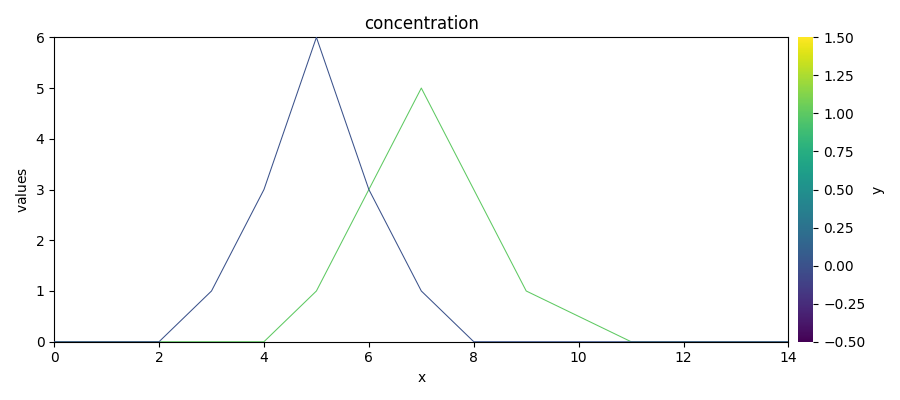
1) simulated chromatogram

t = scp.Coord.arange(15, units="minutes", title="time")  # time coordinates
c = scp.Coord(range(2), title="components")  # component coordinates

dsc = scp.zeros((2, 15), dtype=np.float64, coords=[c, t])
dsc[0, 3:8] = [1, 3, 6, 3, 1]  # compound 1
dsc[1, 5:11] = [1, 3, 5, 3, 1, 0.5]  # compound 2

_ = dsc.plot(title="concentration")

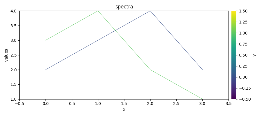
2) absorption spectra

spec = np.array([[2.0, 3.0, 4.0, 2.0], [3.0, 4.0, 2.0, 1.0]])
w = scp.Coord.arange(1, 5, 1, units="nm", title="wavelength")

dss = scp.NDDataset(data=spec, coords=[c, w])
_ = dss.plot(title="spectra")

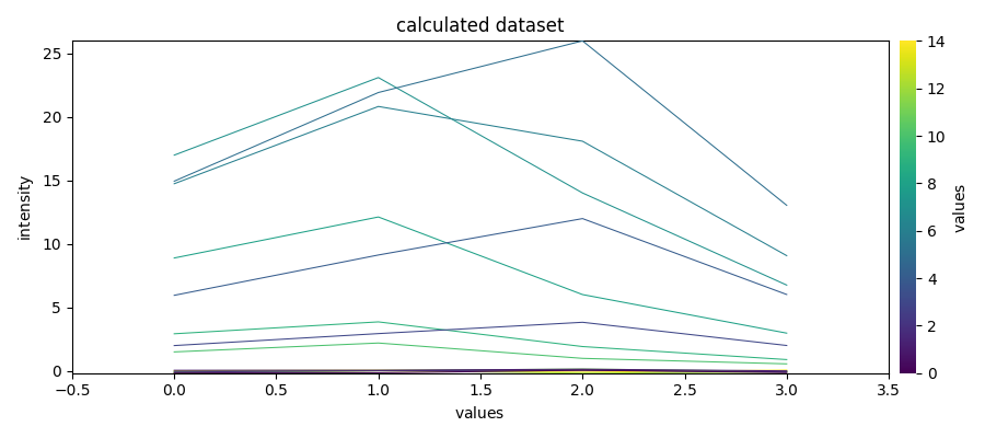
3) simulated data matrix

dataset = scp.dot(dsc.T, dss)
dataset += scp.normal(scale=0.1, size=dataset.shape)
dataset.title = "intensity"

_ = dataset.plot(title="calculated dataset")

4) evolving factor analysis (EFA)

efa = scp.EFA()
_ = efa.fit(dataset)

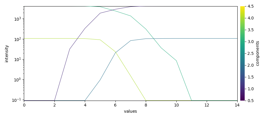
Plots of the log(EV) for the forward and backward analysis

_ = efa.f_ev.T.plot(yscale="log", legend=efa.f_ev.k.labels)

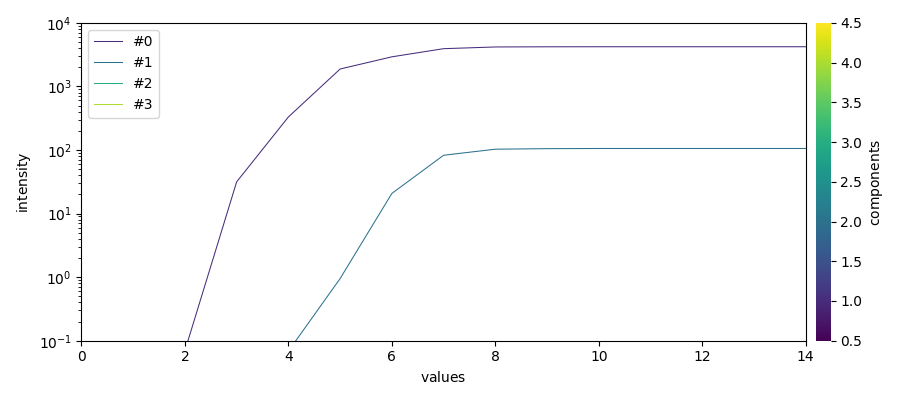
_ = efa.b_ev.T.plot(yscale="log", legend=efa.b_ev.k.labels)

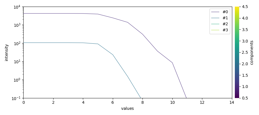
Looking at these EFA curves, it is quite obvious that only two components are really significant, and this corresponds to the data that we have in input. We can consider that the third EFA components is mainly due to the noise, and so we can use it to set a cut of values

n_pc = efa.n_components = 2

efa.cutoff = efa.f_ev[:, n_pc].max()
f2 = efa.f_ev[:, :n_pc]
b2 = efa.b_ev[:, :n_pc]

plot forward and backward EFA curves together without concatenating datasets, which would emit a coordinate warning here.

_ = f2.T.plot(yscale="log")
_ = b2.T.plot(yscale="log", clear=False)

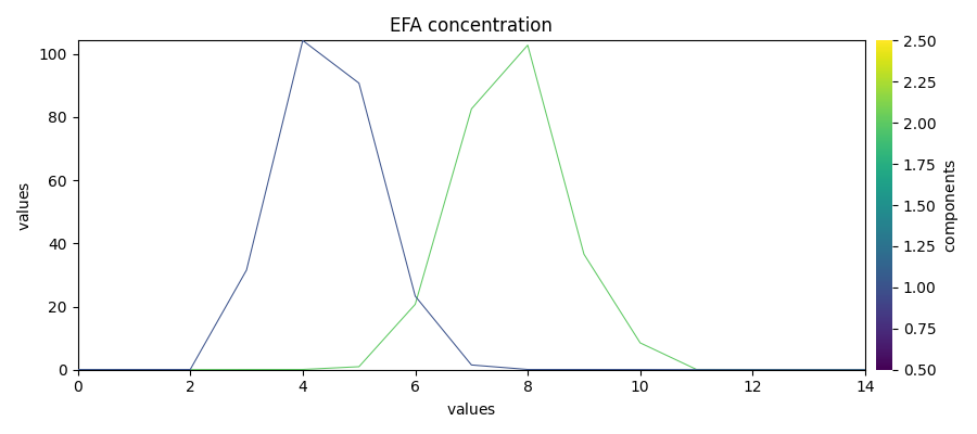
Get the abstract concentration profile based on the FIFO EFA analysis

C = efa.transform()
_ = C.T.plot(title="EFA concentration")

This ends the example ! The following line can be uncommented if no plot shows when running the .py script with python

# scp.show()

Total running time of the script: (0 minutes 1.297 seconds)