Basic transformations
Let’s show some SpectroChemPy features on a group of IR spectra
[1]:
import spectrochempy as scp
from spectrochempy import MASKED
from spectrochempy import DimensionalityError
from spectrochempy import error_
[2]:
dataset = scp.read_omnic("irdata/nh4y-activation.spg")
dataset.y -= dataset.y[0]
dataset.y.title = "time"
dataset
[2]:
NDDataset [nh4y-activation] — float64, shape: (y:55, x:5549), a.u.
Omnic filename: /home/runner/.spectrochempy/testdata/irdata/nh4y-activation.spg
2026-08-25 14:26:22+00:00> Sorted by date
Data
[ 2.033 2.037 ... 1.913 1.911]
...
[ 1.794 1.791 ... 1.198 1.198]
[ 1.816 1.815 ... 1.24 1.238]] a.u.
Dimension `x`
Dimension `y`
[ vz0466.spa, Wed Jul 06 21:00:38 2016 (GMT+02:00) vz0467.spa, Wed Jul 06 21:10:38 2016 (GMT+02:00) ...
vz0520.spa, Thu Jul 07 06:00:41 2016 (GMT+02:00) vz0521.spa, Thu Jul 07 06:10:41 2016 (GMT+02:00)]]
[3]:
prefs = scp.preferences
prefs.figure.figsize = (6, 3)
prefs.colormap = "Dark2"
prefs.colorbar = True
ax = dataset.plot()
Masking data
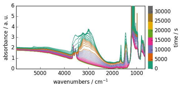
if we try to get for example the maximum of this dataset, we face a problem due to the saturation around 1100 cm\(^{-1}\).
[4]:
dataset.max()
[4]:
One way is to apply the max function to only a part of the spectrum (using slicing). Another way is to mask the undesired data.
Masking values in this case is straightforward. Just set a value masked or True for those data you want to mask.
[5]:
dataset[:, 1290.0:890.0] = MASKED
# note that we specify floating values in order to sect wavenumbers, not index.
Here is a display the figure with the new mask
[6]:
_ = dataset.plot_stack()
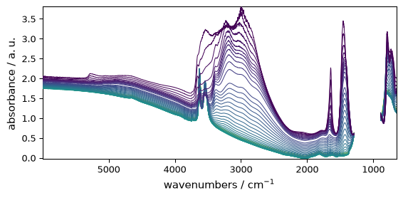
Now the max function return the maximum in the unmasked region, which is exactly what we wanted.
[7]:
dataset.max()
[7]:
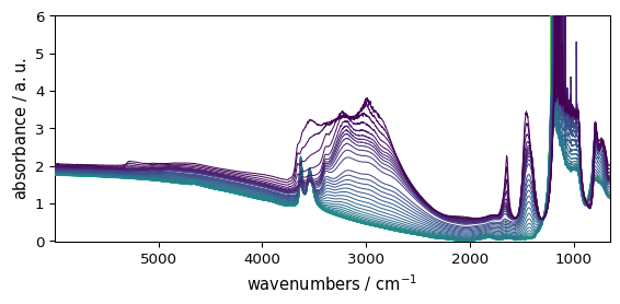
To clear this mask, we can simply do:
[8]:
dataset.remove_masks()
_ = dataset.plot()
Transposition
Dataset can be transposed
[9]:
dataset[:, 1290.0:890.0] = MASKED  # we mask the unwanted columns
t_dataset = dataset.T
t_dataset
[9]:
NDDataset [nh4y-activation] — float64, shape: (x:5549, y:55), a.u.
Omnic filename: /home/runner/.spectrochempy/testdata/irdata/nh4y-activation.spg
2026-08-25 14:26:22+00:00> Sorted by date
2026-08-25 14:26:23+00:00> Data transposed
Data
[ 2.061 2.037 ... 1.791 1.815]
...
[ 2.013 1.913 ... 1.198 1.24]
[ 2.012 1.911 ... 1.198 1.238]] a.u.
Dimension `x`
Dimension `y`
[ vz0466.spa, Wed Jul 06 21:00:38 2016 (GMT+02:00) vz0467.spa, Wed Jul 06 21:10:38 2016 (GMT+02:00) ...
vz0520.spa, Thu Jul 07 06:00:41 2016 (GMT+02:00) vz0521.spa, Thu Jul 07 06:10:41 2016 (GMT+02:00)]]
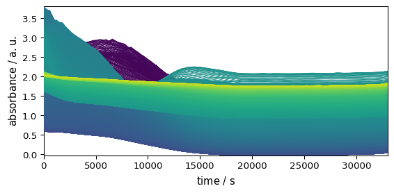
As it can be observed the dimension xand yhave been exchanged, e.g. the original shape was (x: 5549, y: 55), and after transposition it is (y:55, x:5549). (the dimension names stay the same, but the index of the corresponding axis are exchanged).
Let’s visualize the result:
[10]:
_ = t_dataset.plot()
Changing units
Units of the data and coordinates can be changed, but only towards compatible units. For instance, data are in absorbance units, which are dimensionless (a.u). So a dimensionless units such as radian is allowed, even if in this case it makes very little sense.
[11]:
dataset.units = "radian"
[12]:
_ = dataset.plot()
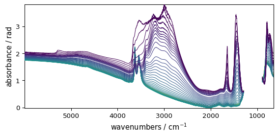
Trying to change it in ‘meter’ for instance, will generate an error!
[13]:
try:
    dataset.to("meter")
except DimensionalityError as e:
    error_(DimensionalityError, e)
ERROR | DimensionalityError: Cannot convert from 'radian' (dimensionless) to 'meter' ([length])
If this is for some reasons something you want to do, you must for the change:
[14]:
d = dataset.to("meter", force=True)
d.units
INFO | units forced to change
[14]:
When units are compatible there is no problem to modify it. For instance, we can change the y dimension units ( Time) to hours. Her we use the inplace transformation ito .
[15]:
dataset.y.ito("hours")
_ = dataset.plot()
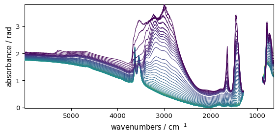
See Units for more details on these units operations
Chemometric preprocessing
SpectroChemPy provides standard preprocessing operations commonly used in chemometrics and spectroscopic data analysis. They operate along a chosen dimension and respect masks, units, coordinates, and metadata.
[16]:
# Load a dataset and focus on a small region for clarity
ds = scp.read_omnic("irdata/nh4y-activation.spg")
ds = ds[:, 4000.0:2000.0]
Normalization
normalize scales data along a dimension. The default method is 'max'.
[17]:
nd = ds.normalize(method="max", dim="x")
_ = nd.plot(title="Max-normalized spectra")
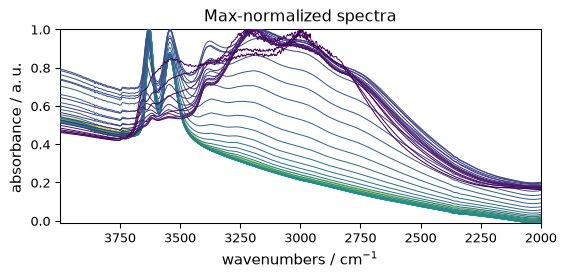
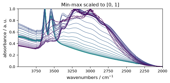
Other methods include 'sum', 'vector' (L2 norm), and 'minmax'.
[18]:
nd = ds.normalize(method="minmax", dim="x")
_ = nd.plot(title="Min-max scaled to [0, 1]")
Mean-centering and autoscaling
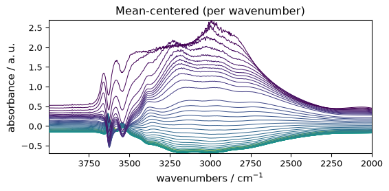
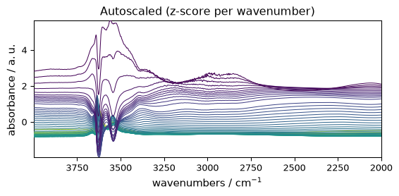
center subtracts the mean. autoscale mean-centres and divides by the standard deviation (z-score). By default these operate per variable (dim='y'), which is the convention before PCA or PLS.
[19]:
nd = ds.center(dim="y")
_ = nd.plot(title="Mean-centered (per wavenumber)")
[20]:
nd = ds.autoscale(dim="y")
_ = nd.plot(title="Autoscaled (z-score per wavenumber)")
Standard Normal Variate (SNV)
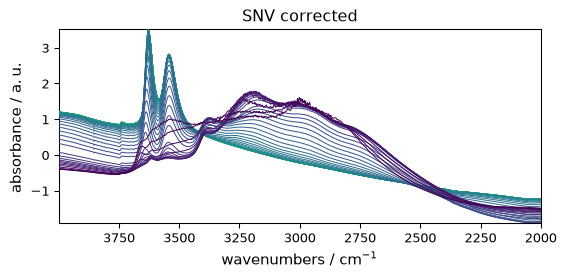
SNV is equivalent to autoscaling each spectrum individually (dim='x'). It is a classic NIR preprocessing step.
[21]:
nd = ds.snv()
_ = nd.plot(title="SNV corrected")
Multiplicative Scatter Correction (MSC)
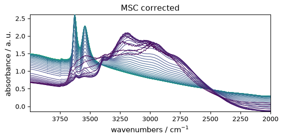
MSC corrects for multiplicative and additive scattering effects by linearly regressing each spectrum against a reference (the mean spectrum by default). In transformer workflows, MSCTransformer.fit() learns only the reference spectrum. The intercept and slope remain local to each transformed spectrum, so inverse_transform() is intentionally unsupported.
[22]:
nd = ds.msc()
_ = nd.plot(title="MSC corrected")
Using transformers for machine-learning workflows
For train/test splits or cross-validation, transformer classes make preprocessing state explicit. Feature-wise scalers reuse statistics learned from a training set:
scaler = scp.AutoscaleTransformer(dim="y")
X_train_scaled = scaler.fit_transform(X_train)
X_test_scaled  = scaler.transform(X_test)   # uses train mean/std
Sample-local operations such as SNVTransformer, NormalizeTransformer(dim="x"), and the per-spectrum regression step in MSCTransformer still compute each observation’s statistics during transform(), because those statistics belong to the spectrum being transformed rather than to the training set. Their inverse transform is not supported unless a future API carries the required per-observation state on the transformed result.
All nine operations have a matching transformer (e.g. CenterTransformer, NormalizeTransformer, MSCTransformer, …). They implement the familiar fit() / transform() / fit_transform() / inverse_transform() lifecycle where meaningful and expose get_params() / set_params() for scikit-learn-compatible cloning.
All operations support inplace=True and can be called as either top-level functions (scp.normalize(...)) or dataset methods (dataset.normalize(...)).