Time domain baseline correction (NMR)

Here we show how to baseline correct dataset in the time domain before applying FFT.

The example spectra were downloaded from this page where you can find some explanations on this kind of process.

[1]:

import spectrochempy as scp

[2]:

# This example uses Bruker NMR data.
#
# Requires the official ``spectrochempy-nmr`` plugin.
# Install with: ``pip install spectrochempy[nmr]``.

[3]:

path = scp.preferences.datadir / "nmrdata" / "bruker" / "tests" / "nmr" / "h3po4"
fid = scp.nmr.read_topspin(path, expno=4)
prefs = scp.preferences
prefs.figure.figsize = (7, 3)
_ = fid.plot(show_complex=True)

../../_images/userguide_processing_td_baseline_3_1.png

[4]:

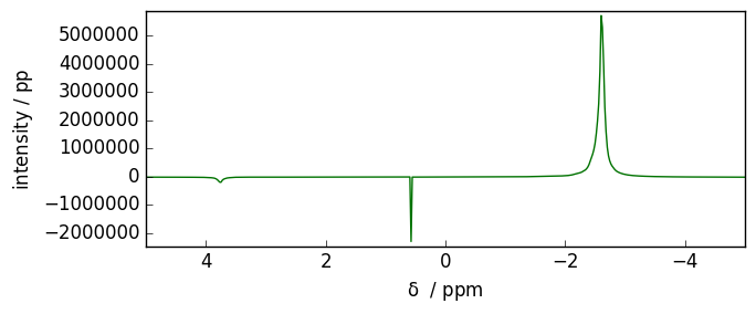
spec = scp.fft(fid)
_ = spec.plot(xlim=(5, -5))

 WARNING | (RuntimeWarning) divide by zero encountered in log10
 WARNING | (RuntimeWarning) divide by zero encountered in scalar divide

../../_images/userguide_processing_td_baseline_4_1.png

We can see that in the middle of the spectrum there are an artifact (a transmitter spike) due to different DC offset between imaginary.

In SpectroChemPy, for now, we provide a simple kind of dc correction using the dccommand.

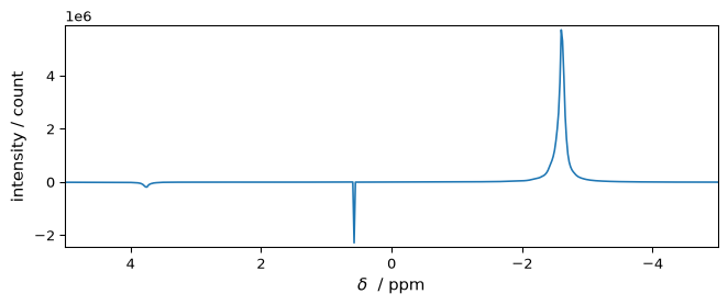
[5]:

dc_corrected_fid = fid.dc()
spec = scp.fft(dc_corrected_fid)
_ = spec.plot(xlim=(5, -5))

 WARNING | (RuntimeWarning) divide by zero encountered in log10
 WARNING | (RuntimeWarning) divide by zero encountered in scalar divide

../../_images/userguide_processing_td_baseline_6_1.png

[6]:

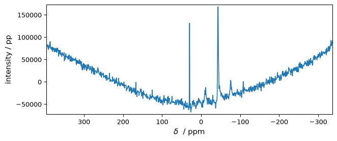
path = scp.preferences.datadir / "nmrdata" / "bruker" / "tests" / "nmr" / "cadmium"
fid2 = scp.nmr.read_topspin(path, expno=100)
_ = fid2.plot(show_complex=True)

 WARNING | (UserWarning) (956,)cannot be shaped into(1024,)

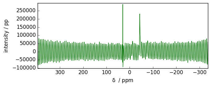
../../_images/userguide_processing_td_baseline_7_1.png

[7]:

spec2 = scp.fft(fid2)
_ = spec2.plot()

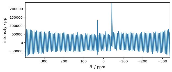
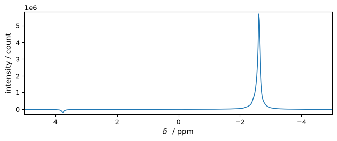
../../_images/userguide_processing_td_baseline_8_0.png

[8]:

dc_corrected_fid2 = fid2.dc()
spec2 = scp.fft(dc_corrected_fid2)
_ = spec2.plot()

../../_images/userguide_processing_td_baseline_9_0.png