Note
Go to the end to download the full example code.
Fitting 1D dataset
In this example, we find the least square solution of a simple linear equation.
import os

import spectrochempy as scp
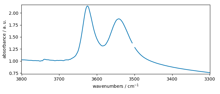
Let’s take an IR spectrum
nd = scp.read_omnic(os.path.join("irdata", "nh4y-activation.spg"))
and select only the OH region:
Perform a Fit Fit parameters are defined in a script (a single text as below)
script = """
#-----------------------------------------------------------
# syntax for parameters definition:
# name: value, low_bound,  high_bound
# available prefix:
#  # for comments
#  * for fixed parameters
#  $ for variable parameters
#  > for reference to a parameter in the COMMON block
#    (> is forbidden in the COMMON block)
# common block parameters should not have a _ in their names
#-----------------------------------------------------------
#

COMMON:
# common parameters ex.
# $ gwidth: 1.0, 0.0, none
$ gratio: 0.1, 0.0, 1.0

MODEL: LINE_1
shape: asymmetricvoigtmodel
    * ampl:  1.1, 0.0, none
    $ pos:   3620, 3400.0, 3700.0
    $ ratio: 0.0147, 0.0, 1.0
    $ asym: 0.1, 0, 1
    $ width: 50, 0, 1000

MODEL: LINE_2
shape: asymmetricvoigtmodel
    $ ampl:  0.8, 0.0, none
    $ pos:   3540, 3400.0, 3700.0
    > ratio: gratio
    $ asym: 0.1, 0, 1
    $ width: 50, 0, 1000

"""
create an Optimize object
f1 = scp.Optimize(log_level="INFO")
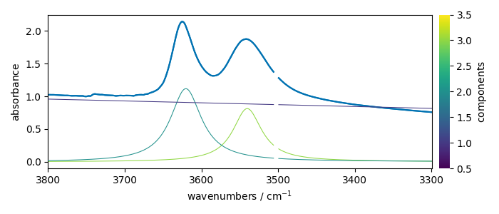
Show plot and the starting model using the dry parameters (of course it is advisable to be as close as possible of a good expectation
f1.script = script

# set dry and continue to show starting model
# reset dry and continue to show starting model
f1.dry = True
f1.autobase = True
f1.fit(ndOH)

# get some information
scp.info_(f"numbers of components: {f1.n_components}")
_ = ndOH.plot()
ax = (f1.components[:]).plot(clear=False)
ax.autoscale(enable=True, axis="y")
**************************************************
Starting parameters:
**************************************************

COMMON:
       $ gratio:     0.1000, 0.0, 1.0

MODEL: line_1
shape: asymmetricvoigtmodel
       * ampl:     1.1000, 0.0, none
       $ asym:     0.1000, 0, 1
       $ pos:  3620.0000, 3400.0, 3700.0
       $ ratio:     0.0147, 0.0, 1.0
       $ width:    50.0000, 0, 1000

MODEL: line_2
shape: asymmetricvoigtmodel
       $ ampl:     0.8000, 0.0, none
       $ asym:     0.1000, 0, 1
       $ pos:  3540.0000, 3400.0, 3700.0
       > ratio:gratio
       $ width:    50.0000, 0, 1000

numbers of components: 2
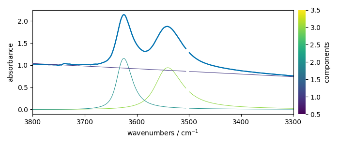
Now perform a fit with maximum 1000 iterations
f1.max_iter = 1000
f1.fit(ndOH)
 **************************************************
 Result:
 **************************************************

 COMMON:
        $ gratio:     0.3458, 0.0, 1.0

 MODEL: line_1
 shape: asymmetricvoigtmodel
        * ampl:     1.1000, 0.0, none
        $ asym:     0.7716, 0, 1
        $ pos:  3623.4044, 3400.0, 3700.0
        $ ratio:     0.4394, 0.0, 1.0
        $ width:    43.5995, 0, 1000

 MODEL: line_2
 shape: asymmetricvoigtmodel
        $ ampl:     0.9001, 0.0, none
        $ asym:     1.0000, 0, 1
        $ pos:  3536.9977, 3400.0, 3700.0
        > ratio:gratio
        $ width:    79.4888, 0, 1000


<spectrochempy.analysis.curvefitting.optimize.Optimize object at 0x7fc57deb2060>
Show the result
_ = ndOH.plot()
ax = (f1.components[:]).plot(clear=False)
ax.autoscale(enable=True, axis="y")
plotmerit
som = f1.inverse_transform()
f1.plotmerit(ndOH, som, method="scatter", markevery=5, markersize=2, lw=2)
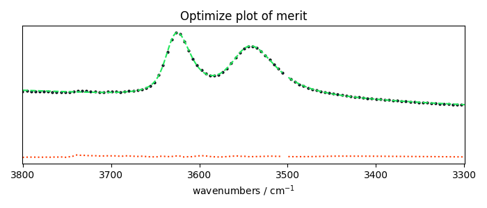
<Axes: xlabel='wavenumbers $\\mathrm{/\\ \\mathrm{cm}^{-1}}$', ylabel='absorbance $\\mathrm{/\\ \\mathrm{a.u.}}$'>
This ends the example ! The following line can be uncommented if no plot shows when running the .py script with python
# scp.show()
Total running time of the script: (0 minutes 1.084 seconds)