× ⚠️ You are reading the development version documentation.
Read here the documentation of the last stable release.

Processing RAMAN spectra

Various examples of processing RAMAN spectra

Import API

import spectrochempy as scp

Importing a 1D spectra

Define the folder where are the spectra

datadir = scp.preferences.datadir
ramandir = datadir / "ramandata/labspec"

Read a single spectrum

A = scp.read_labspec("SMC1-Initial_RT.txt", directory=ramandir)

Plot the spectrum

A.plot()

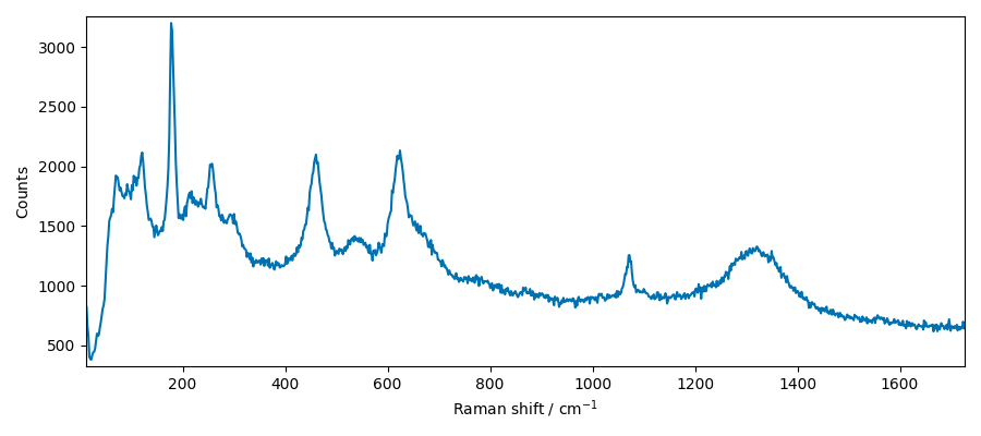
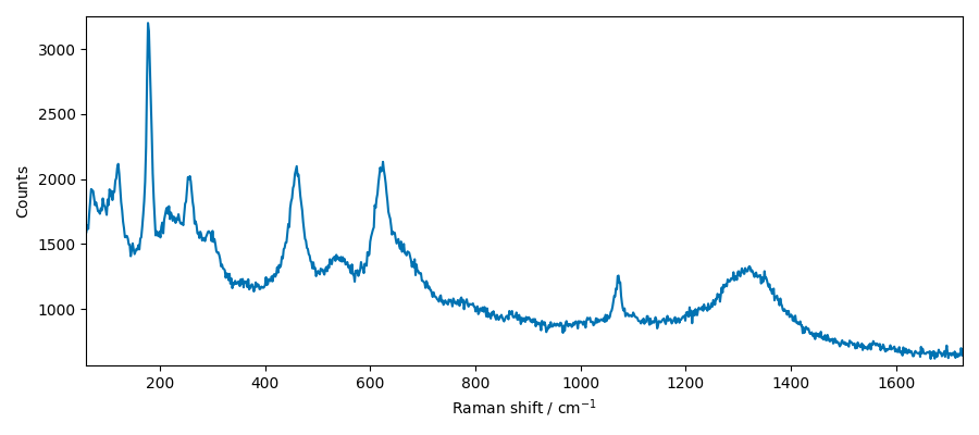
Crop the spectrum to a useful region

B = A[60.0:]
B.plot()

Baseline correction

Let’s try to remove the baseline using different methods For this we use the Baseline processor

First, we define the baseline processor

blc = scp.Baseline(log_level="INFO")

Now we can try the various baseline methods.

Detrending

the detrend method is not strictly speaking a method to calculate a bottom line, but it can be useful as a preprocessing to remove a trend. Let’s define the model to be used for detrending

blc.model = "detrend"

Now we need to define the order of the detrending either as an integer giving the degree of the polynomial trend or a string among { constant , linear , quadratic , cubic }

blc.order = "linear"

Now we can fit the model to the data

blc.fit(B)

<spectrochempy.processing.baselineprocessing.baselineprocessing.Baseline object at 0x7fcff1f91f50>

The baseline is now stored in the baseline attribute of the processor

corr = blc.transform()
baseline = blc.baseline

Let’s plot the result of the correction

As we will use this type of plot several times, we define a function for it

def plot_result(X, Xc, bas):
    Xcm = Xc.min()
    Xcp = Xc.ptp()
    offset = Xcm + Xcp
    (Xc - Xcm).plot()
    (X + offset).plot(clear=False, color="g", linestyle="-")
    (bas + offset).plot(clear=False, color="r", linestyle="--")


plot_result(B, corr, baseline)

Let’s try with a polynomial detrend of order 2

blc.order = 2  # quadratic detrending
blc.fit(B)
corr = blc.transform()
baseline = blc.baseline
plot_result(B, corr, baseline)

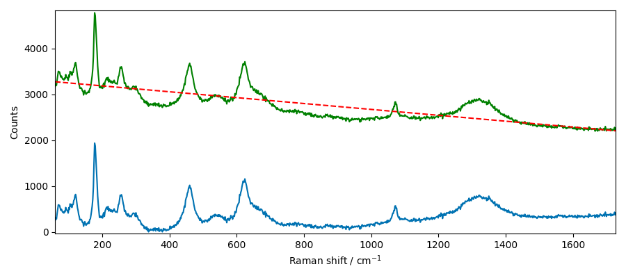
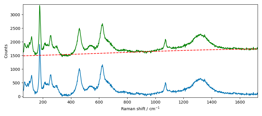
Ok this is a good start. But we can do better with more specific baseline correction methods. Let’s try the asymmetric least squares smoothing model ( asls ), on this detrended spectrum:

Bd = blc.corrected

Asymmetric Least Squares smoothing

blc.model = "asls"

We need to define the smoothness and asymmetry parameters. The smoothness parameter is a positive number that controls the smoothness of the baseline. The larger this number is, the smoother the resulting baseline. The asymmetry parameter controls the asymmetry for the AsLS resolution.

blc.lamb = 10**8  # smoothness
blc.asymmetry = 0.01

Now we can fit the model to the data

blc.fit(Bd)
corr = blc.transform()
baseline = blc.baseline
plot_result(Bd, corr, baseline)

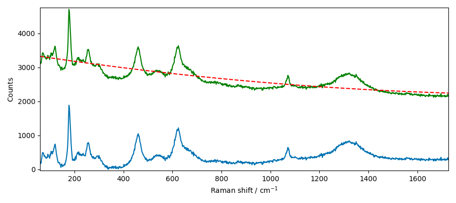
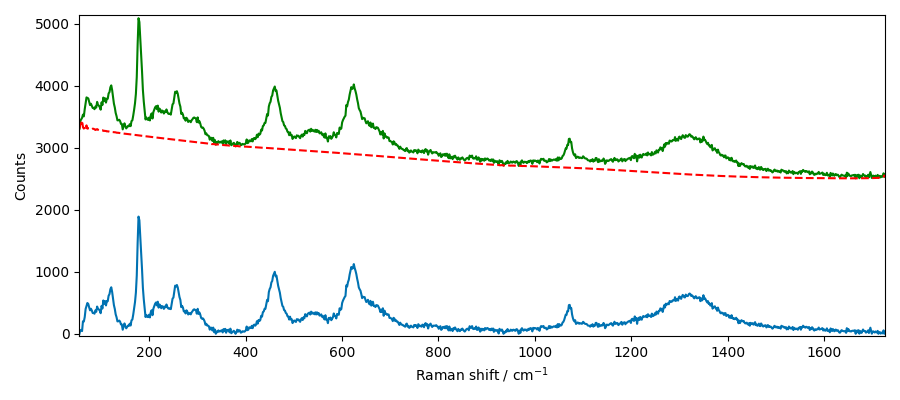
The correction appears to be good, but let’s see if we can do better by using the snip method. This method requires to adjust the width of a window (usually set to the FWHM of the characteristic peaks).

blc.model = "snip"
blc.snip_width = 55  # estimated FWHM of the peaks (expressed in point. TODO: alternatively use true coordinates)
Bs = A[55.0:]
blc.fit(Bs)
corr = blc.transform()
baseline = blc.baseline
plot_result(Bs, corr, baseline)

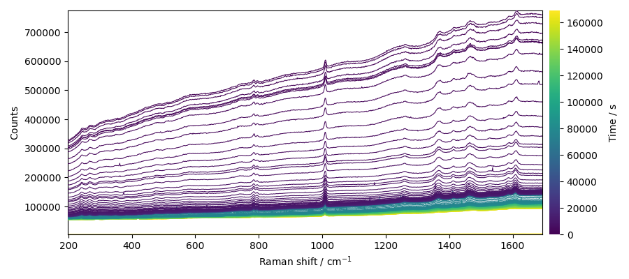
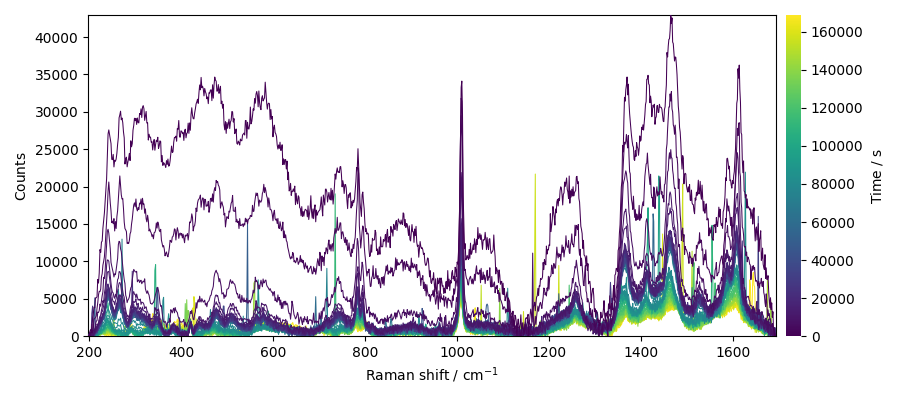
Baseline correction 2D spectra (series of spectra)

First, we read the series of spectra

C = scp.read_labspec("Activation.txt", directory=ramandir)
# C = C[20:]  # discard the first 20 spectra
C.plot()

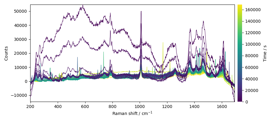
Now we apply the AsLS method on the series of spectra

We keep the same parameters as before and fit the new dataset The baseline is calculated for each spectrum of the series. So the process is very slow! For the demonstration we will the limit the series to 1 spectrum over 10.

blc.model = "asls"
blc.log_level = (
    "WARNING"  # supress output of asls (to long for the moment:  TODO optimize this)
)
blc.fit(C[::10])
corr = blc.transform()
baseline = blc.baseline
corr.plot()

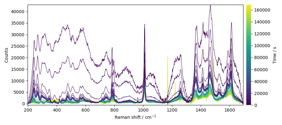
or the snip method (which is much faster)

blc.model = "snip"
blc.fit(C)
corr = blc.transform()
baseline = blc.baseline
corr[::10].plot()

Denoising

D = corr.copy()
G = scp.denoise(D, ratio=98)

G[::10].plot()

This ends the example ! The following line can be removed or commented when the example is run as a notebook (ipynb).

# scp.show()