× ⚠️ You are reading the development version documentation.
Read here the documentation of the last stable release.

MCR-ALS example (adapted from Jaumot et al. 2005)

In this example, we perform the MCR ALS optimization of a dataset corresponding to a HPLC-DAD run, from Jaumot et al. [2005] and Jaumot et al. [2015].

This dataset (and others) can be downloaded from the Multivariate Curve Resolution Homepage.

For the user convenience, this dataset is present in the test data directory scp.preferences.datadir of SpectroChemPy as als2004dataset.MAT.

Import the spectrochempy API package

import spectrochempy as scp

Loading the example dataset

The file type (matlab) is inferred from the extension .mat, so we can use the generic API function read. Alternatively, one can be more specific by using the read_matlab function. Both have exactly the same behavior.

datasets = scp.read("matlabdata/als2004dataset.MAT")

As the .mat file contains 6 matrices, 6 NDDataset objects are returned.

print("NDDataset names:")
for ds in datasets:
    print(f"{ds.name} : {ds.shape}")

NDDataset names:
cpure : (204, 4)
MATRIX : (204, 96)
isp_matrix : (4, 4)
spure : (4, 96)
csel_matrix : (51, 4)
m1 : (51, 96)

We are interested in the last dataset ("m1") that contains a single HPLS-DAD run (51x96) dataset.

As usual, the 51 rows correspond to the time axis of the HPLC run, and the 96 columns to the wavelength axis of the UV spectra. The original dataset does not contain information as to the actual time and wavelength coordinates.

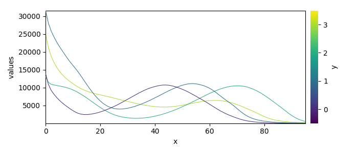
MCR-ALS needs also an initial guess for either concentration profiles or pure spectra concentration profiles. The 4th dataset in the example ("spure") contains (4x96) guess of spectral profiles.

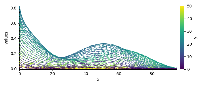
The experimental data as \(X\) (X) and the guess are thus:

X = datasets[-1]
guess = datasets[3]

Plot of X and of the guess:

X.plot()
guess.plot()

• 
• 

Create a MCR-ALS object

We first create a MCR-ALS object named here mcr.

The log_level option can be set to "INFO" to get verbose ouput of the MCR-ALS optimization steps.

mcr = scp.MCRALS(log_level="INFO")

Fit the MCR-ALS model

Then we execute the optimization process using the fit method with the X and guess dataset as input arguments.

mcr.fit(X, guess)

<spectrochempy.analysis.decomposition.mcrals.MCRALS object at 0x7f0091874ec0>

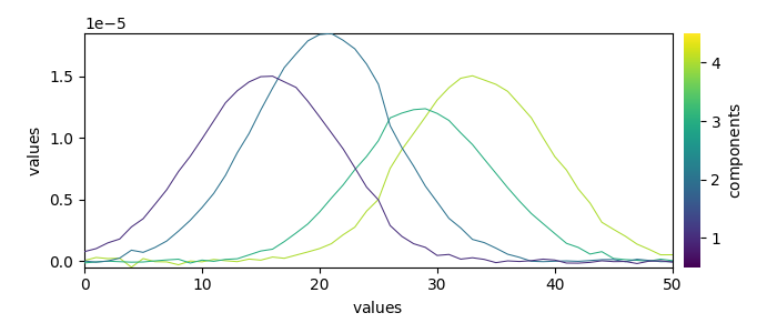
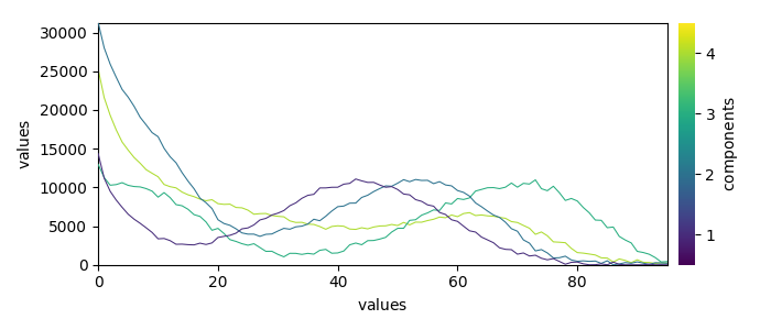
Plotting the results

The optimization has converged. We can get the concentration \(C\) (C) and pure spectra profiles \(S^T\) (St) and plot them

mcr.C.T.plot()
mcr.St.plot()

• 
• 

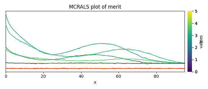
Finally, plots the reconstructed dataset (\(\hat{X} = C.S^T\)) vs. original dataset (\(X\)) as well as the residuals (\(E\)) for few spectra.

The fit is good and comparable to the original paper (Jaumot et al. [2005]).

mcr.plotmerit(nb_traces=5)

This ends the example ! The following line can be uncommented if no plot shows when running the .py script with python

# scp.show()