MCR-ALS: Multivariate Curve Resolution with Alternating Least Squares
This tutorial covers three progressively complex MCR-ALS workflows:
Classical MCR-ALS — a single HPLC-DAD experiment;
Constraints — incorporating prior chemical knowledge;
Augmented datasets — vertical (multi-experiment) and horizontal (multi-technique) data fusion.
Each part answers a practical question the reader is likely to ask. The goal is to teach the methodology, not to enumerate every API feature.
Part I — Classical MCR-ALS
The bilinear model
MCR-ALS decomposes an experimental data matrix \(X\) into the product of two physically interpretable factor matrices:
where:
\(C\) contains the concentration profiles of the pure species (rows → observations (time), columns → components (species));
\(S^T\) contains the pure spectra (rows → components (species), columns → spectral variables (wavelengths));
\(E\) is the residual.
The ALS algorithm iteratively estimates \(C\) from \(S^T\) and \(S^T\) from \(C\) subject to constraints, until the improvement in the fit falls below a tolerance.
1. Loading and inspecting the data
We use the ALS2004 benchmark dataset from Jaumot et al., Chemolab, 76 (2005) 101–110 and Chemolab, 140 (2015) 1–12. It contains HPLC-DAD measurements of a mixture of four co-eluting species.
[1]:
import spectrochempy as scp

datasets = scp.read("matlabdata/als2004dataset.MAT")
for d in datasets:
    print(f"{d.name}: {d.shape}")
cpure: (204, 4)
MATRIX: (204, 96)
isp_matrix: (4, 4)
spure: (4, 96)
csel_matrix: (51, 4)
m1: (51, 96)
We select the first chromatographic run (m1, 51 × 96) which contains the experimental data and the published pure-component spectra (spure, 4 × 96) which will be used to initialize the MCRALS.
[2]:
X = datasets[-1]
St0 = datasets[3]

X.title = "absorbance"
X.set_coordset(None, None)
X.set_coordtitles(y="elution time", x="wavelength")

_ = X.plot(title="experimental spectra")
_ = St0.plot(title="pure-component spectra")
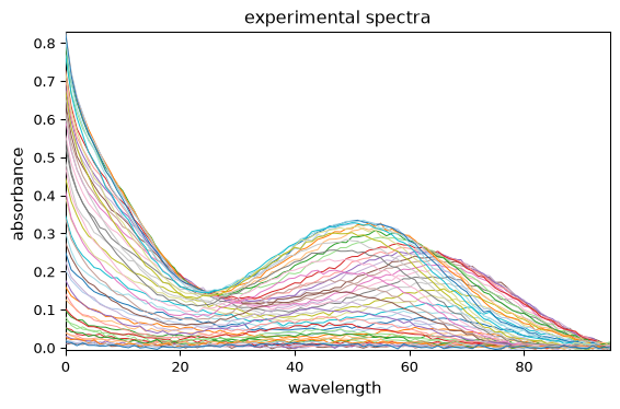
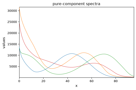
The 51 rows of Xare elution times; the 96 columns are wavelengths. Overlapping bands cannot be resolved by inspection alone — this is where curve resolution is needed.
2. How many components? — PCA
Principal Component Analysis (PCA) can be used to estimate the number of components. In particular a scree plot of the PCA eigenvalues is often used to provide a quick estimate of the effective rank.
[3]:
pca = scp.PCA(n_components=8)
pca.fit(X)
_ = pca.plot_scree()
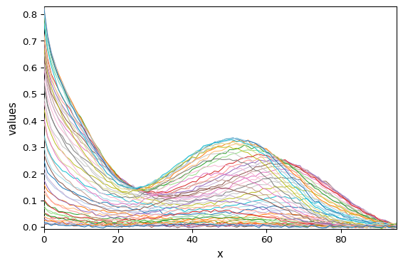
The scree plot suggests that the effective rank is likely between three and four components. The fourth component explains only a small fraction of the total variance, so PCA alone does not provide an unambiguous choice. The EFA analysis below can give additional information and supports the use of four components for the MCR-ALS model.
3. Where do the components appear? — Evolving Factor Analysis
PCA estimates the overall rank of the dataset but does not indicate where individual chemical components are present along the elution axis. Evolving Factor Analysis (EFA) addresses this question by performing a sequence of singular value decompositions (or equivalently PCA) on progressively larger submatrices of the data.
In the forward analysis, the decomposition is performed on submatrices extending from the beginning of the experiment to each observation in turn. In the backward analysis, the same procedure is applied starting from the last observation and extending progressively towards the beginning.
The evolution of the significant eigenvalues reflects changes in the local rank of the system. It reveals where chemical components enter and leave the observation window, providing both an estimate of the number of components and approximate bounds for their elution regions.
[4]:
efa = scp.EFA()
efa.fit(X)

# Plot forward and backward eigenvalue curves on a log scale
scp.log10(efa.f_ev.clip(1e-4)).T.plot(color="dodgerblue")
_ = scp.log10(efa.b_ev.clip(1e-4)).T.plot(clear=False, color="limegreen")
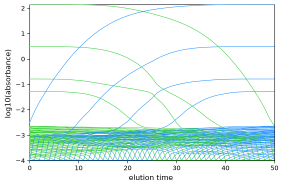
Four eigenvalues rise clearly above the noise floor. The forward curve (blue) for each component marks its emergence; the backward curve (green) marks its decline. The zone where the \(k\)-th forward curve separates from the noise is the elution window of component \(k\).
From these windows, EFA constructs approximate concentration profiles that describe where each component is present along the chromatogram. Although these profiles are only estimates, they provide, in this case, an excellent initialization for MCR-ALS.
[5]:
efa.n_components = 4
C0 = efa.transform()

_ = C0.T.plot()
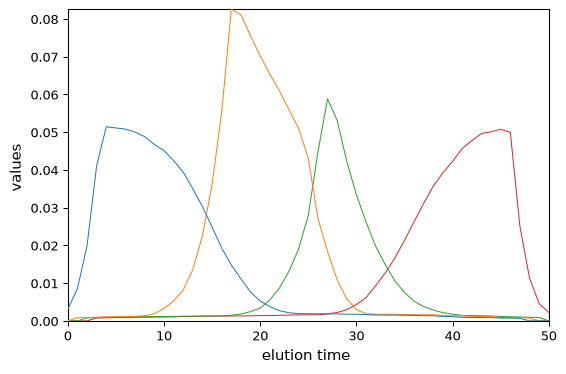
EFA provides a physically meaningful initial estimate: each profile naturally respects the elution order and peak shape implied by the data. It is particularly effective for systems that evolve sequentially along the observation axis, such as chromatographic separations where components elute in a first-in, first-out order (it was actually initially developed for this purpose).
4. Other initialization methods
Several other strategies exist:
SIMPLISMA — selects purest variables as initial spectra;
Known reference spectra — when pure-component spectra have been measured independently (e.g. in a spectral library);
Known concentration profiles — when the elution or kinetic model is known a priori.
In this tutorial we will use successively the pure spectra spure as the initial \(S^T\) (stored in St0) and the EFA initialization as the initial \(C\) (stored in C0). and compare the two approaches.
5. Running the optimisation
The default configuration already applies non-negativity to both \(C\) and \(S^T\), and unimodality to \(C\) — sensible defaults for chromatographic data.
Let’s first run the MCR-ALS algorithm with the pure spectra as initial guess for \(S^T\).
[6]:
mcr_s = scp.MCRALS(log_level="INFO")
_ = mcr_s.fit(X, St0)
 Spectra profile initialized with 4 components
 Initial concentration profile computed
 ***                         ALS optimisation log                         ***
 #iter  reconstruction_error  residual_change  profile_change  trend
 -----------------------------------------------------------------------
     1          1.748031e-02     9.764498e-01    2.329779e-02   down
     2          1.745947e-02     9.620502e-04    4.201766e-03   down
 Converged on residual_change:
   residual_change=9.620502e-04 <= tol_residual_change=1.000000e-03
6. Inspecting the solution
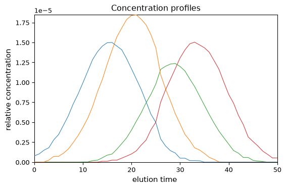
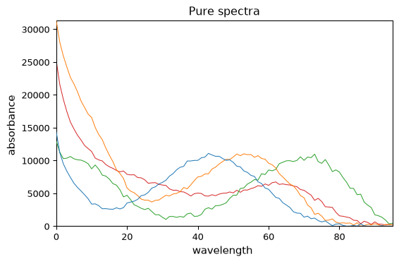
The estimated profiles preserve the coordinate metadata of the input data.
[7]:
C = mcr_s.C
St = mcr_s.St

print(f"C: {C.shape}")
print(f"St: {St.shape}")

_ = C.T.plot(title="Concentration profiles")
_ = St.plot(title="Pure spectra")
C: (51, 4)
St: (4, 96)
The reconstruction quality can be assessed with plot_merit:
[8]:
_ = mcr_s.plot_merit(offset=5)
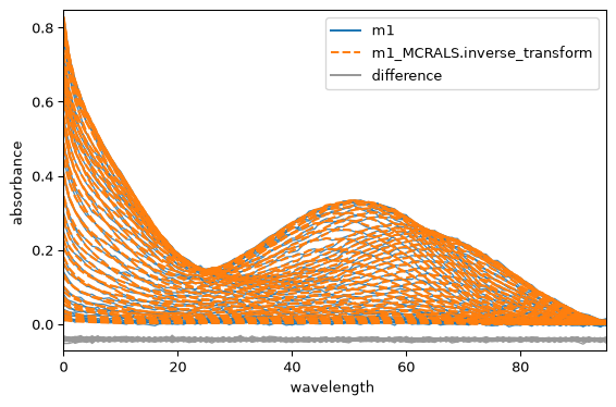
Numerical diagnostics confirm convergence:
[9]:
print(f"Residual std: {mcr_s.result.diagnostics['residual_std']:.6f}")
print(f"Converged: {mcr_s.result.converged}")
print(f"Iterations: {mcr_s.result.n_iter}")
Residual std: 0.002932
Converged: True
Iterations: 2
Now let’s run the MCR-ALS algorithm with the EFA initialization for \(C\) and the pure spectra as initial guess for \(S^T\) and compare the two approaches. %%0 mcr_c = scp.MCRALS(log_level=”INFO”) _ = mcr_c.fit(X, C0)
import matplotlib.pyplot as plt
fig, axes = plt.subplots(nrows=3, ncols=2, figsize=(8, 6)) mcr_c.C.T.plot(ax=axes[0, 0], title=”C (EFA init)”) mcr_s.C.T.plot(ax=axes[0, 1], title=”C (Pure spectra init)”) mcr_c.St.plot(ax=axes[1, 0], title=”\(S^T\) (EFA init)”) mcr_s.St.plot(ax=axes[1, 1], title=”\(S^T\) (Pure spectra init)”) mcr_c.plot_merit(ax=axes[2, 0], offset=5) mcr_s.plot_merit(ax=axes[2, 1], offset=5) plt.tight_layout() plt.show()
The EFA initializations converges less rapidly but provides very similar reconstruction, as shown by the comparable residuals in the merit plots. This indicates that the bilinear model describes the experimental data consistently, regardless of whether the initial estimate is supplied for \(C\) or for \(S^T\).
Note, however, that the amplitudes of the resolved profiles differ substantially. This reflects the intrinsic scale ambiguity of MCR-ALS: multiplying one column of \(C\) by a constant and dividing the corresponding row of \(S^T\) by the same constant leaves the product \(CS^T\) unchanged. Consequently, the absolute magnitudes of the concentration and spectral profiles should not be compared directly unless a common normalization convention is imposed.
Differences are also observed in the shapes of the resolved profiles. These arise because EFA provides only an approximate initial estimate and because the spectra of several components overlap strongly. Such spectral correlation makes the decomposition less well conditioned, allowing slightly different distributions of variance between components while producing nearly identical reconstructions of the experimental data. This behaviour is typical of bilinear inverse problems and illustrates why chemically meaningful constraints are often essential to obtain a unique and interpretable solution.
Part II — Constraints
The true power of MCR-ALS lies in the ability to inject prior chemical knowledge through constraints. SpectroChemPy provides a declarative constraint API: each constraint is a simple object that describes what is known.
The most important practical question is: which constraint should I use for my scientific problem?
Quick reference
The constraints are imported from spectrochempy.analysis.constraints:
Constraint |
Profile |
Purpose |
|---|---|---|
|
C, St |
Non-negativity of concentrations or spectra |
|
C, St |
Single maximum per component (chromatography, kinetics) |
|
C |
Constant sum of selected components (mass balance) |
|
C |
Monotonic increase or decrease (kinetic or thermodynamic profiles) |
|
C, St |
Hard model from a user-supplied callable (kinetic model) |
|
C |
Component absent in certain blocks (augmented data) |
|
C |
Rank-1 constraint across blocks (augmented data) |
All constraints accept optional blocks= (see below) and components= parameters to restrict their scope.
Non-negativity
Non-negativity is the most widely used constraint in MCR-ALS because both chemical concentrations and absorbance spectra are inherently non-negative. For this reason, the default MCR-ALS configuration in SpectroChemPy applies this constraint automatically to both concentration and spectral profiles.
To illustrate its effect, we first remove all constraints and solve the problem using unconstrained least squares
[10]:
mcr_nc = scp.MCRALS(log_level="INFO", constraints=[])
mcr_nc.fit(X, C0)
_ = mcr_nc.C.T.plot(title="Non-constrained concentration profiles")
 Concentration profile initialized with 4 components
 Initial spectra profile computed
 ***                         ALS optimisation log                         ***
 #iter  reconstruction_error  residual_change  profile_change  trend
 -----------------------------------------------------------------------
     1          1.665088e-02     9.775524e-01    4.647900e-01   down
     2          1.665003e-02     5.127431e-05    3.022884e-03   down
 Converged on residual_change:
   residual_change=5.127431e-05 <= tol_residual_change=1.000000e-03
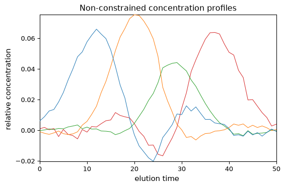
The unconstrained least-squares solution contains negative concentrations and oscillatory profiles.
How is non-negativity enforced?
There are two common strategies for enforcing non-negativity during the ALS iterations.
The default configuration follows the classical MCR-ALS strategy introduced by Tauler and co-workers: each ALS half-step first computes an unconstrained least-squares solution:
after which the NonNegative constraint then projects this solution onto the non-negative domain by replacing negative values with zero:
This approach is computationally inexpensive. Here we demonstrate this for concentrations:
[11]:
from spectrochempy.analysis import constraints as ct

mcr_nn = scp.MCRALS(log_level="INFO", constraints=[ct.NonNegative("C")])
mcr_nn.fit(X, C0)
_ = mcr_nn.C.T.plot(title="Non-negative concentration profiles (projection)")
 Concentration profile initialized with 4 components
 Initial spectra profile computed
 ***                         ALS optimisation log                         ***
 #iter  reconstruction_error  residual_change  profile_change  trend
 -----------------------------------------------------------------------
     1          5.767978e-02     9.232964e-01    4.397632e-01   down
     2          4.043192e-02     3.043839e-01    5.692102e-02   down
     3          3.283399e-02     1.906242e-01    2.949484e-02   down
     4          2.862415e-02     1.288964e-01    1.862694e-02   down
     5          2.604415e-02     8.943053e-02    1.363284e-02   down
     6          2.429795e-02     6.529846e-02    1.054868e-02   down
     7          2.310245e-02     4.746912e-02    8.422678e-03   down
     8          2.221190e-02     3.696109e-02    6.956822e-03   down
     9          2.151895e-02     2.980714e-02    5.841260e-03   down
    10          2.096108e-02     2.467126e-02    5.029301e-03   down
    11          2.050065e-02     2.083361e-02    4.383544e-03   down
    12          2.011751e-02     1.763101e-02    3.858344e-03   down
    13          1.979623e-02     1.505146e-02    3.461305e-03   down
    14          1.952482e-02     1.288648e-02    3.152172e-03   down
    15          1.929219e-02     1.114532e-02    2.894323e-03   down
    16          1.909267e-02     9.613618e-03    2.661589e-03   down
    17          1.892095e-02     8.299861e-03    2.449585e-03   down
    18          1.877223e-02     7.194934e-03    2.259211e-03   down
    19          1.864378e-02     6.224673e-03    2.085434e-03   down
    20          1.853283e-02     5.379301e-03    1.925637e-03   down
    21          1.843679e-02     4.681179e-03    1.779336e-03   down
    22          1.835306e-02     4.098826e-03    1.648279e-03   down
    23          1.828088e-02     3.553773e-03    1.530151e-03   down
    24          1.821690e-02     3.160191e-03    1.424304e-03   down
    25          1.816000e-02     2.807360e-03    1.327170e-03   down
    26          1.810926e-02     2.499969e-03    1.237831e-03   down
    27          1.806269e-02     2.339595e-03    1.164532e-03   down
    28          1.801850e-02     2.240620e-03    1.115006e-03   down
    29          1.797636e-02     2.146093e-03    1.097718e-03   down
    30          1.793619e-02     2.049510e-03    1.081548e-03   down
    31          1.789785e-02     1.958642e-03    1.064975e-03   down
    32          1.786125e-02     1.872664e-03    1.048070e-03   down
    33          1.782629e-02     1.791172e-03    1.030910e-03   down
    34          1.779288e-02     1.713830e-03    1.013573e-03   down
    35          1.776095e-02     1.640348e-03    9.961340e-04   down
    36          1.773041e-02     1.570471e-03    9.786633e-04   down
    37          1.770120e-02     1.503974e-03    9.612273e-04   down
    38          1.767324e-02     1.440657e-03    9.438864e-04   down
    39          1.764649e-02     1.380339e-03    9.266953e-04   down
    40          1.762087e-02     1.322855e-03    9.097028e-04   down
    41          1.759634e-02     1.268054e-03    8.929519e-04   down
    42          1.757284e-02     1.215797e-03    8.764799e-04   down
    43          1.755032e-02     1.165956e-03    8.603191e-04   down
    44          1.752880e-02     1.118744e-03    8.446747e-04   down
    45          1.750816e-02     1.073807e-03    8.293799e-04   down
    46          1.748836e-02     1.030876e-03    8.144415e-04   down
    47          1.746936e-02     9.898752e-04    7.998752e-04   down
 Converged on residual_change:
   residual_change=9.898752e-04 <= tol_residual_change=1.000000e-03
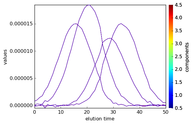
Alternatively, the least-squares problem itself can be solved under the non-negativity constraint,
using a dedicated non-negative least-squares (NNLS) solver. In this case, positivity is enforced during the least-squares optimization rather than by projecting an unconstrained solution afterwards. The resulting estimate is the exact non-negative least-squares solution, at the expense of a higher computational cost.
The choice of solver is independent of the constraint definition. The NonNegative constraint specifies that the solution must be non-negative, whereas the ALS solver determines whether this constraint is enforced by projection (lstsq) or directly during the optimization (nnls or pnnls).
Here we demonstrate the nnls solver for concentrations:
[12]:
from spectrochempy.analysis import constraints as ct

mcr_nnl = scp.MCRALS(log_level="INFO", solver_C="nnls", constraints=[])

mcr_nnl.fit(X, C0)
_ = mcr_nnl.C.T.plot(title="Non-negative concentration profiles (NNSL solver)")
 Concentration profile initialized with 4 components
 Initial spectra profile computed
 ***                         ALS optimisation log                         ***
 #iter  reconstruction_error  residual_change  profile_change  trend
 -----------------------------------------------------------------------
     1          1.826900e-02     9.753740e-01    4.722650e-01   down
     2          1.748447e-02     4.294342e-02    5.962034e-02   down
     3          1.720964e-02     1.571503e-02    3.230377e-02   down
     4          1.706891e-02     8.170357e-03    2.175036e-02   down
     5          1.698353e-02     4.994049e-03    1.622493e-02   down
     6          1.693017e-02     3.132939e-03    1.232892e-02   down
     7          1.689353e-02     2.153603e-03    9.858229e-03   down
     8          1.686519e-02     1.669704e-03    8.367374e-03   down
     9          1.684238e-02     1.344693e-03    7.307099e-03   down
    10          1.682403e-02     1.082754e-03    6.394584e-03   down
    11          1.680924e-02     8.737452e-04    5.590653e-03   down
 Converged on residual_change:
   residual_change=8.737452e-04 <= tol_residual_change=1.000000e-03
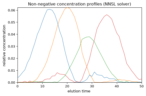
Here we obtain non-negative concentration profiles without projection. Note however that some profiles are not unimodal – this point will be addressed in a following section.
Below we show how to apply non-negativity constraints particular profiles:
[13]:
# All concentration profiles (default)
_ = ct.NonNegative("C")

# All spectral profiles (default)
_ = ct.NonNegative("St")

# Selected concentration components
_ = ct.NonNegative("C", components=[0, 1])

# Selected spectral components
_ = ct.NonNegative("St", components=[0])

# Selected blocks of an augmented dataset (see below)
_ = ct.NonNegative("C", blocks=[1, 2])
_ = ct.NonNegative("St", blocks=[0])  # e.g. UV spectra only

# Combine component and block selections
_ = ct.NonNegative("C", components=[0], blocks=[2])
Constraints are supplied as a list when constructing the MCR-ALS estimator.
[14]:
mcr = scp.MCRALS(
    constraints=[
        ct.NonNegative("C"),
        ct.NonNegative(
            "St", blocks=[0]
        ),  # e.g. only the first block has non-negative spectra
    ],
    log_level="INFO",
)
Unimodality
In chromatography or kinetics each concentration profile typically has a single maximum.
[15]:
_ = ct.Unimodal("C", mod="strict")  # strict single maximum (default)
_ = ct.Unimodal("C", mod="smooth")  # allows a flat-topped region
_ = ct.Unimodal("C", tolerance=1.0)  # no allowance for local violations
Here we illustrate
mcr_nnl_u = scp.MCRALS( log_level=”INFO”, solver_C=”nnls”, constraints=[ct.Unimodal(“C”)] )
mcr_nnl_u.fit(X, C0) _ = mcr_nnl_u.C.T.plot(title=”NNSL solver + unimodality”)
Unimodality can also be applied to spectral profiles when thy consist in a single band:
[16]:
_ = ct.Unimodal("St", components=[1]) # only the second component
Closure
Useful when the total concentration of the mixture is known.
[17]:
_ = ct.Closure("C")  # rows sum to 1.0
_ = ct.Closure("C", target=100.0)  # custom constant sum
_ = ct.Closure("C", target=[1.0, 0.9, 0.8])  # per-row targets
Monotonic
For kinetic profiles that only increase or decrease.
[18]:
_ = ct.Monotonic("C", "increasing", components=[0])
_ = ct.Monotonic("C", "decreasing", components=[1])
ModelProfile
When a profile shape is known from a physical model (kinetic rate law, peak-shape function), the ALS estimate is replaced by the model output at each iteration.
[19]:
# def kinetic_model(C_current):
#     return C_constrained
#
# ct.ModelProfile("C", model=kinetic_model)
ComponentPresence
For augmented (multi-block) data: specify which components are present in each concentration block.
[20]:
# ct.ComponentPresence("C", presence=[
#     [True, True, True, True],
#     [True, True, True, False],
# ])
Trilinear — the rank-one assumption
Trilinearity is the only constraint we demonstrate in full because it addresses a recurring question in multi-experiment MCR-ALS.
When the same mixture is measured repeatedly under identical conditions (e.g. several HPLC injections), each component should have the same concentration profile shape across runs, differing only by a per-experiment amplitude. Mathematically, the concentration profiles of each component form a rank‑1 matrix across experiments:
where \(a\) is the common shape and \(b\) contains the amplitudes. The Trilinear constraint enforces this by projecting the per-component, multi-block profiles onto their best rank‑1 approximation at every ALS iteration.
Repeated chromatographic runs of the same mixture naturally satisfy this assumption. The constraint is applied during vertical augmentation, which we cover in the next section.
A practical note: the default MCR-ALS configuration already applies NonNegative and Unimodal to the concentration profiles, so explicitly adding these constraints will barely change the ALS2004 solution. They are the first constraints to consider for any new dataset; the more specialised constraints above become relevant when the default model needs refinement.
Part III — Augmented datasets
MCR-ALS can simultaneously analyse multiple data matrices. SpectroChemPy supports two augmentation modes, each corresponding to a different scientific scenario.
A. Vertical augmentation — multiple experiments, common spectra
In vertical (column-wise) augmentation several experiments are stacked row-wise. Each experiment has its own concentration profiles, but the pure spectra \(S^T\) are common to all.
The ALS2004 dataset contains the MATRIX variable: four successive HPLC-DAD runs concatenated into a single 204 × 96 matrix.
[21]:
X2 = datasets[1]
X2.title = "absorbance"
X2.set_coordset(None, None)
X2.set_coordtitles(y="elution time", x="wavelength")

X_blocks = [X2[i * 51 : (i + 1) * 51].copy() for i in range(4)]
for i, b in enumerate(X_blocks):
    b.name = f"run {i + 1}"
    b.title = "absorbance"
    print(f"{b.name}: {b.shape}")
run 1: (51, 96)
run 2: (51, 96)
run 3: (51, 96)
run 4: (51, 96)
The blocks share the same spectral variables (96 wavelengths) but have their own elution-time axes. When all blocks have identical dimensions (51 × 96), we must specify augmentation="vertical" explicitly.
[22]:
mcr_v = scp.MCRALS(log_level="INFO")
_ = mcr_v.fit(X_blocks, St0, augmentation="vertical")
 Spectra profile initialized with 4 components
 Initial concentration profile computed
 ***                         ALS optimisation log                         ***
 #iter  reconstruction_error  residual_change  profile_change  trend
 -----------------------------------------------------------------------
     1          2.037383e-02     9.726990e-01    1.120336e-02   down
     2          2.034643e-02     1.113181e-03    2.790146e-03   down
     3          2.034542e-02     2.950587e-05    1.345692e-03     up
 Converged on residual_change:
   residual_change=2.950587e-05 <= tol_residual_change=1.000000e-03
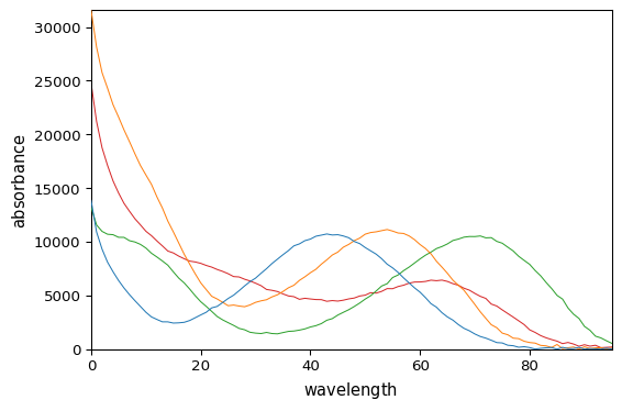
The concentration matrix is the row-wise concatenation of the individual \(C_k\) blocks. The C_blocks property restores the per-experiment view:
[23]:
print(f"C (concatenated): {mcr_v.C.shape}")
print(f"St (common): {mcr_v.St.shape}")

for i, cb in enumerate(mcr_v.C_blocks):
    print(f"C_blocks[{i}]: {cb.shape}")
C (concatenated): (204, 4)
St (common): (4, 96)
C_blocks[0]: (51, 4)
C_blocks[1]: (51, 4)
C_blocks[2]: (51, 4)
C_blocks[3]: (51, 4)
[24]:
_ = scp.multiplot(
    [cb.T for cb in mcr_v.C_blocks],
    nrow=2,
    ncol=2,
    suptitle="Concentration profiles — vertical augmentation",
)
Trilinearity
Repeated chromatographic runs of the same mixture should produce concentration profiles with identical shapes, differing only in scale. We can enforce this with the Trilinear constraint.
[25]:
mcr_vt = scp.MCRALS(
    constraints=[ct.NonNegative("C"), ct.NonNegative("St"), ct.Trilinear("C")],
    log_level="INFO",
)
_ = mcr_vt.fit(X_blocks, St0, augmentation="vertical")
 Spectra profile initialized with 4 components
 Initial concentration profile computed
 ***                         ALS optimisation log                         ***
 #iter  reconstruction_error  residual_change  profile_change  trend
 -----------------------------------------------------------------------
     1          2.013676e-02     9.730370e-01    1.644983e-02   down
     2          2.013830e-02     1.968120e-05    1.726896e-03     up
 Converged on residual_change:
   residual_change=1.968120e-05 <= tol_residual_change=1.000000e-03
For the ALS2004 benchmark, the four runs are already highly consistent profiles (cross-block correlations > 0.998), so the constraint does not substantially change the fit:
[26]:
print(
    f"Without trilinearity — residual std: {mcr_v.result.diagnostics['residual_std']:.4f}"
)
print(
    f"With trilinearity    — residual std: {mcr_vt.result.diagnostics['residual_std']:.4f}"
)

_ = scp.multiplot(
    [cb.T for cb in mcr_vt.C_blocks],
    nrow=2,
    ncol=2,
    suptitle="Concentration profiles — trilinear constraint",
)
Without trilinearity — residual std: 0.0030
With trilinearity    — residual std: 0.0030
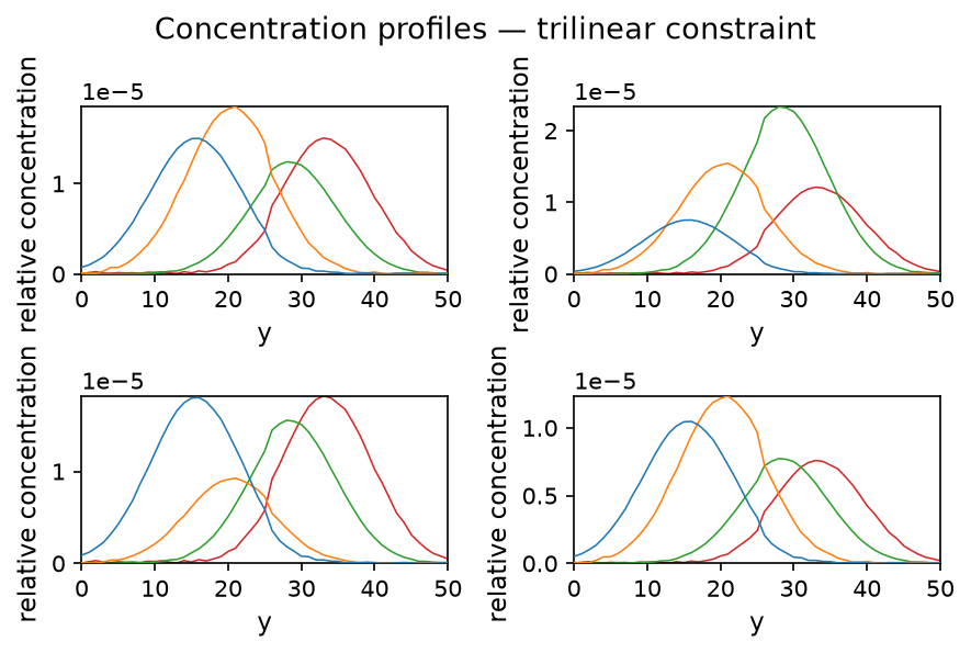
The value of the Trilinear constraint becomes apparent with noisier data or when runs exhibit slight instrumental drift. In those cases, forcing a common shape removes artefactual differences and produces chemically more interpretable profiles.
B. Horizontal augmentation — common observations, different spectroscopies
In horizontal (row-wise) augmentation several data matrices share the observation axis (same number of rows) but have different spectral variables. The concentration profiles \(C\) are common, while each technique contributes its own spectral block \(S_i^T\).
This is useful when the same sample is measured with complementary spectroscopic techniques — the joint analysis forces a single concentration profile to explain all techniques simultaneously.
Building two complementary spectral blocks
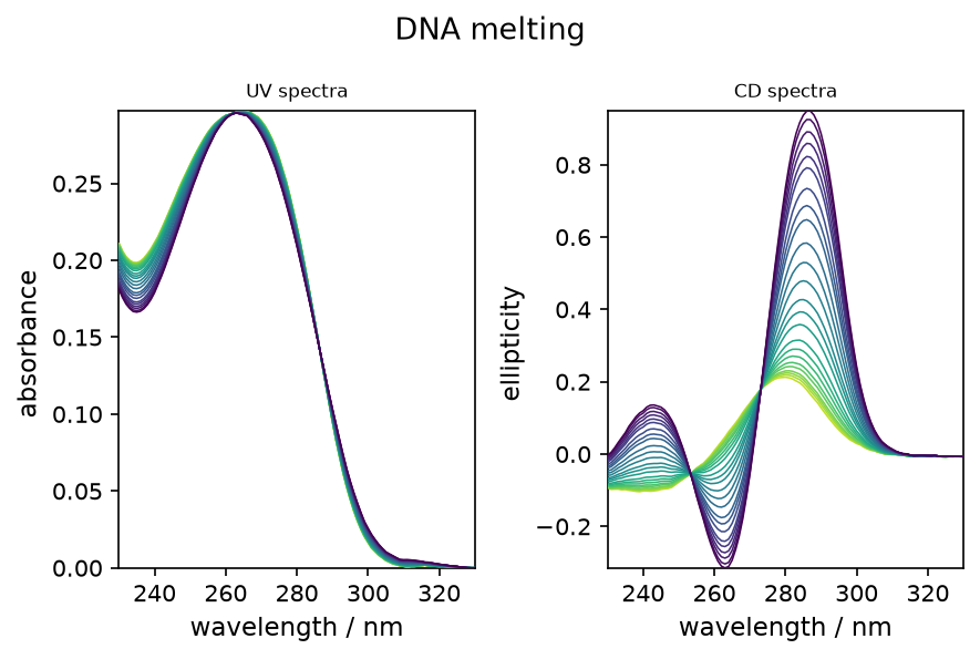
To keep this tutorial fully reproducible in offline test environments, we derive a horizontal-augmentation example from the ALS2004 benchmark itself. We split the wavelength axis into two complementary blocks:
a left block containing the lower wavelengths, kept as ordinary non-negative absorbance data;
a right block that we mean-center row-wise to mimic a signed measurement channel where positive and negative bands coexist.
[27]:
split_index = X.shape[1] // 2

X_uv = X[:, :split_index].copy()
X_uv.name = "Block A"
X_uv.title = "absorbance"
X_uv.x.title = "wavelength"

X_cd = X[:, split_index:].copy()
X_cd.name = "Block B"
X_cd.title = "centered absorbance"
X_cd.x.title = "wavelength"
X_cd.data = X_cd.data - X_cd.data.mean(axis=1, keepdims=True)

print(f"{X_uv.name}: {X_uv.shape}")
print(f"{X_cd.name}: {X_cd.shape}")
Block A: (51, 48)
Block B: (51, 48)
[28]:
_ = scp.multiplot(
    (X_uv, X_cd),
    nrow=1,
    ncol=2,
    labels=("Block A", "Block B"),
    suptitle="Horizontal augmentation example",
)
Building a deterministic initial guess
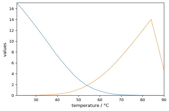
We use an EFA-based initialization on the combined UV+CD data.
[29]:
# concatenate the two datasets
combined = scp.concatenate(
    X_uv, X_cd
)  # a warning is raised because we concatenate absorbances and ellipticities

# fit an EFA
efa = scp.EFA().fit(combined)

# and plot forward and backward curves to deternamlibne
scp.log10(efa.f_ev.clip(1e-5)).T.plot(color="dodgerblue")
_ = scp.log10(efa.b_ev.clip(1e-5)).T.plot(clear=False, color="limegreen")
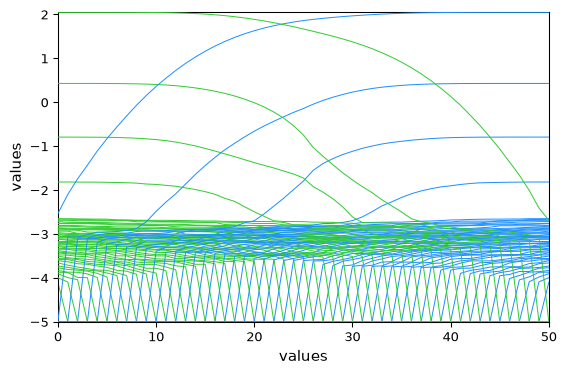
The plot above still supports a four-component model, consistent with the original ALS2004 decomposition.
[30]:
efa.n_components = 4
C0 = efa.transform()
_ = C0.T.plot()
Choosing the right constraints
The first block is non-negative, but the mean-centered second block is signed (positive and negative bands), so global non-negativity on \(S^T\) would be incorrect.
We therefore apply NonNegative only to the first spectral block (block 0):
[31]:
mcr_h = scp.MCRALS(
    constraints=[
        ct.NonNegative("C"),
        ct.NonNegative("St", blocks=[0]),
        ct.Closure("C"),
    ],
    log_level="INFO",
    tol_reconstruction_error=1e-3,
)
_ = mcr_h.fit([X_uv, X_cd], C0, augmentation="horizontal")
 Concentration profile initialized with 4 components
 Initial spectra profile computed
 ***                         ALS optimisation log                         ***
 #iter  reconstruction_error  residual_change  profile_change  trend
 -----------------------------------------------------------------------
     1          5.584081e-02     9.366873e-01    5.052967e-01   down
     2          3.935780e-02     2.971169e-01    5.507597e-02   down
     3          3.214258e-02     1.846137e-01    2.775240e-02   down
     4          2.849084e-02     1.140131e-01    1.725419e-02   down
     5          2.643925e-02     7.190737e-02    1.219663e-02   down
     6          2.509120e-02     5.067479e-02    9.614492e-03   down
     7          2.416164e-02     3.661748e-02    7.787844e-03   down
     8          2.349518e-02     2.712106e-02    6.462814e-03   down
     9          2.299655e-02     2.074050e-02    5.540009e-03   down
    10          2.260980e-02     1.636082e-02    4.890526e-03   down
    11          2.229110e-02     1.373277e-02    4.420817e-03   down
    12          2.201671e-02     1.196337e-02    4.036883e-03   down
    13          2.177813e-02     1.050844e-02    3.702609e-03   down
    14          2.157034e-02     9.228092e-03    3.402364e-03   down
    15          2.138938e-02     8.094259e-03    3.127234e-03   down
    16          2.123136e-02     7.108651e-03    2.875748e-03   down
    17          2.109290e-02     6.261720e-03    2.646553e-03   down
    18          2.097113e-02     5.530819e-03    2.436491e-03   down
    19          2.086387e-02     4.889716e-03    2.243953e-03   down
    20          2.076977e-02     4.309583e-03    2.072300e-03   down
    21          2.068564e-02     3.864260e-03    1.920838e-03   down
    22          2.061026e-02     3.470247e-03    1.782688e-03   down
    23          2.054256e-02     3.123677e-03    1.656687e-03   down
    24          2.048107e-02     2.857537e-03    1.544748e-03   down
    25          2.042380e-02     2.683001e-03    1.455773e-03   down
    26          2.036996e-02     2.538044e-03    1.379069e-03   down
    27          2.032009e-02     2.359964e-03    1.319149e-03   down
    28          2.027340e-02     2.214645e-03    1.279263e-03   down
    29          2.022940e-02     2.093283e-03    1.243727e-03   down
    30          2.018721e-02     2.024224e-03    1.215606e-03   down
    31          2.014629e-02     1.967223e-03    1.191975e-03   down
    32          2.010659e-02     1.912156e-03    1.170136e-03   down
    33          2.006806e-02     1.859299e-03    1.149786e-03   down
    34          2.003068e-02     1.808424e-03    1.130698e-03   down
    35          1.999439e-02     1.760016e-03    1.112780e-03   down
    36          1.995913e-02     1.713690e-03    1.095758e-03   down
    37          1.992484e-02     1.668767e-03    1.079474e-03   down
    38          1.989150e-02     1.625236e-03    1.063822e-03   down
    39          1.985908e-02     1.583024e-03    1.048713e-03   down
    40          1.982754e-02     1.542058e-03    1.034076e-03   down
    41          1.979686e-02     1.502270e-03    1.019852e-03   down
    42          1.976702e-02     1.463604e-03    1.005994e-03   down
    43          1.973798e-02     1.426008e-03    9.924637e-04   down
    44          1.970972e-02     1.389438e-03    9.792290e-04   down
    45          1.968223e-02     1.353852e-03    9.662640e-04   down
    46          1.965547e-02     1.319216e-03    9.535474e-04   down
    47          1.962942e-02     1.285494e-03    9.410614e-04   down
    48          1.960408e-02     1.252658e-03    9.287913e-04   down
    49          1.957941e-02     1.220678e-03    9.167248e-04   down
    50          1.955539e-02     1.189529e-03    9.048516e-04   down
 Convergence criterion not reached after  50 iterations.
 Stop ALS optimization.
The concentration profiles \(C\) carry the temperature coordinate. The concatenated spectral matrix \(S^T\) is split into technique-specific blocks via St_blocks, each preserving its own wavelength coordinate.
[32]:
import matplotlib.pyplot as plt

fig, axes = plt.subplots(1, 3, figsize=(12, 4))
_ = mcr_h.C.T.plot(ax=axes[0], title="$C$")
_ = mcr_h.St_blocks[0].plot(ax=axes[1], title="$S^T_1$ (Block A)")
_ = mcr_h.St_blocks[1].plot(ax=axes[2], title="$S^T_2$ (Block B)")
plt.tight_layout()
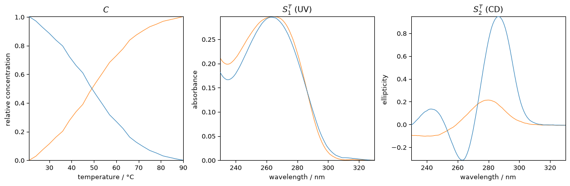
The resolved concentration profiles are shared across both spectral blocks. The first block stays non-negative, while the second retains its signed structure, illustrating why block-specific constraints matter in horizontal augmentation.
Summary — choosing the right workflow
The three parts of this tutorial map directly to practical questions:
One experiment
        │
        ▼
 Classical MCR-ALS
 (Part I)

Repeated experiments
(common spectra)
        │
        ▼
Vertical augmentation
(Part III-A)
        │
        ├── runs are consistent    →  no trilinearity needed
        └── runs need shape alignment → add ct.Trilinear("C")

Multiple techniques
(common concentrations)
        │
        ▼
Horizontal augmentation
(Part III-B)
        │
        └── per-block constraints    →  ct.NonNegative("St", blocks=[...])