[1]:
# ruff: noqa: T201
Quickstart Tutorial 🚀
Contents
What you’ll learn
Load and visualize spectroscopic data
Perform basic data manipulation and plotting
Apply common processing techniques
Use advanced analysis methods
Installing SpectroChemPy
Prerequisites ✅
Python 3.11 or later
Basic knowledge of Python
Jupyter notebook environment
You can install SpectroChemPy using either pip or mamba:
Using pip:
pip install spectrochempy
Using mamba:
mamba install -c spectrocat spectrochempy
See the Installation Guide for detailed instructions.
In the following, we assume that we are running spectrochempy in a Jupyter notebook. See here for details on how to start a Jupyter notebook.
Getting Started
Let’s start by importing SpectroChemPy and checking its version:
[2]:
import spectrochempy as scp
Working with Spectroscopic Data
Loading Data
SpectroChemPy supports many file formats including:
OMNIC (.spa, .spg)
JCAMP-DX (.dx, .jdx)
CSV files
And many more
Let’s load an example FTIR dataset:
[3]:
# Load FTIR data of NH4Y zeolite activation
ds = scp.read("irdata/nh4y-activation.spg")
print(f"Dataset shape: {ds.shape}")  # Show dimensions
print(f"x-axis unit: {ds.x.units}")  # Show wavenumber units
print(f"y-axis unit: {ds.y.units}")  # Show time units
Dataset shape: (55, 5549)
x-axis unit: cm⁻¹
y-axis unit: s
The read function is a powerful method that can load various file formats. In this case, we loaded an OMNIC file. For a full list of supported formats, see the Import tutorial section.
The read function returns an NDDataset object.
Exploring the Data
Understanding the NDDataset object
The NDDataset is the core data structure in SpectroChemPy. It’s designed specifically for spectroscopic data and provides:
Multi-dimensional data support
Coordinates and units handling
Built-in visualization
Processing methods
You can display the loaded NDDataset in a Jupyter notebook as follows:
[4]:
print(ds)
NDDataset: [float64] a.u. (shape: (y:55, x:5549))
Basic information about the data are given in the summary: data type, units, shape, and name of the dataset.
Clicking on the arrow on the left side of the summary will expand the metadata section, which contains additional information about the dataset.
The data itself is contained in the data attribute, which is a numpy array of shape (55,5549).
[5]:
ds.data
[5]:
array([[   2.057,    2.061, ...,    2.013,    2.012],
       [   2.033,    2.037, ...,    1.913,    1.911],
       ...,
       [   1.794,    1.791, ...,    1.198,    1.198],
       [   1.816,    1.815, ...,     1.24,    1.238]], shape=(55, 5549))
The x and y attributes contain the coordinates of the dataset. In this case, the x-axis represents the wavenumber:
[6]:
ds.x
[6]:
Coord [x:wavenumbers] — float64, size: 5549, cm⁻¹
The y-axis represents the sample acquisition time:
[7]:
ds.y
[7]:
Coord [y:acquisition timestamp (GMT)] — float64, size: 55, s
[ vz0466.spa, Wed Jul 06 21:00:38 2016 (GMT+02:00) vz0467.spa, Wed Jul 06 21:10:38 2016 (GMT+02:00) ...
vz0520.spa, Thu Jul 07 06:00:41 2016 (GMT+02:00) vz0521.spa, Thu Jul 07 06:10:41 2016 (GMT+02:00)]]
Data Visualization
SpectroChemPy’s plotting capabilities are built on matplotlib but provide spectroscopy-specific features:
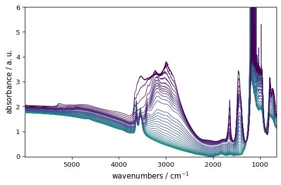
[8]:
_ = ds.plot()
Data Selection and Manipulation
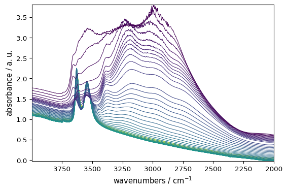
You can easily select specific regions of your spectra using intuitive slicing. Here we select wavenumbers between 4000 and 2000 cm⁻¹:
[9]:
region = ds[:, 4000.0:2000.0]
_ = region.plot()
Mathematical Operations
NDDataset supports various mathematical operations. Here’s an example of basic operations on coordinates and data:
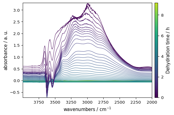
Make y coordinate (time) relative to the first spectrum, convert to hours (default are seconds), and update the title to reflect the new meaning of the y-axis.
[10]:
region.y -= region.y[0]
region.y.ito("hour")
region.y.title = "Dehydration time"
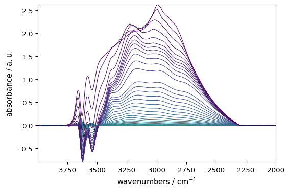
Subtract the last spectrum from all spectra
[11]:
region -= region[-1]
Plot with colorbar to show intensity changes
[12]:
_ = region.plot(colorbar=True)
Other Operations
NDDataset supports many other operations, such as:
Arithmetic operations
Statistical analysis
Data transformation
And more
For more information, see:
API Reference for a full list of available operations.
Plotting tutorial for more information on advanced plotting.
Data Processing Techniques
SpectroChemPy includes numerous processing methods. Here are some common examples:
Spectral Smoothing
Reduce noise while preserving spectral features:
[13]:
smoothed = region.smooth(size=51, window="hanning")
_ = smoothed.plot(colormap="magma")
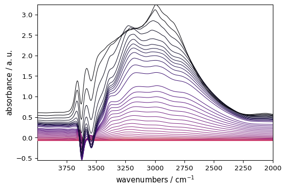
Baseline Correction
Various algorithms are available for baseline correction, including polynomial fitting, rubberband, and more. Here an example of multivariate polynomial baseline correction using PCHIP interpolation is shown:
Configure baseline correction
[14]:
blc = scp.Baseline()
blc.ranges = [[2000.0, 2300.0], [3800.0, 3900.0]]  # Baseline regions
blc.multivariate = True
blc.model = "polynomial"
blc.order = "pchip"
blc.n_components = 5
Apply correction
[15]:
blc.fit(smoothed)
_ = blc.corrected.plot()
SpectroChemPy provides many other processing techniques, such as:
Normalization
Derivatives
Peak detection
And more
For more information, see the Processing tutorial section.
Advanced Analysis
Optional plugin workflows
Some advanced workflows are provided by optional official plugins. For example, 2D-IRIS analysis is available through the spectrochempy-iris plugin and NMR TopSpin reading is available through spectrochempy-nmr. These workflows are documented in the central examples gallery and in the plugin guide, while this quickstart keeps to the standard SpectroChemPy experience.
Other Advanced Analysis Techniques
SpectroChemPy includes many other advanced analysis techniques, such as:
Multivariate analysis
Peak fitting
Kinetic modeling
And more
For more information, see the Advanced Analysis tutorial section.
Next Steps 🎯
Now that you’ve got a taste of SpectroChemPy’s capabilities, here are some suggestions for diving deeper:
Examples Gallery 📈: Browse through practical examples and use cases
User Guide 📖: Learn about specific features in detail
API Reference 🔍: Explore the complete API documentation
Get Help 💬: Join our community discussions