Customizing a Plot

The default plot is designed to look good with minimal effort. However, every visual aspect can be adjusted using keyword arguments passed to ds.plot(). This page covers the most common customizations.

Line Appearance

For 1D and 2D datasets, you can adjust how lines appear:

[1]:

import spectrochempy as scp

ds = scp.read("irdata/nh4y-activation.spg")

Color

[2]:

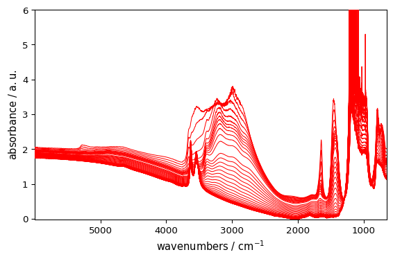
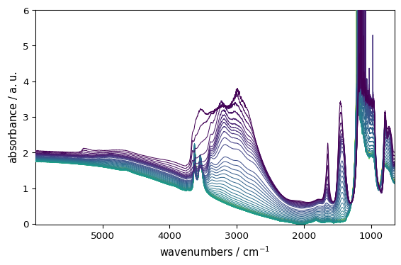
_ = ds.plot(color="red")

../../_images/userguide_plotting_customization_4_0.png

Line Width

[3]:

_ = ds.plot(linewidth=2)

../../_images/userguide_plotting_customization_6_0.png

Line Style

[4]:

_ = ds.plot(linestyle="--")

../../_images/userguide_plotting_customization_8_0.png

Marker

[5]:

_ = ds.plot(marker="o")

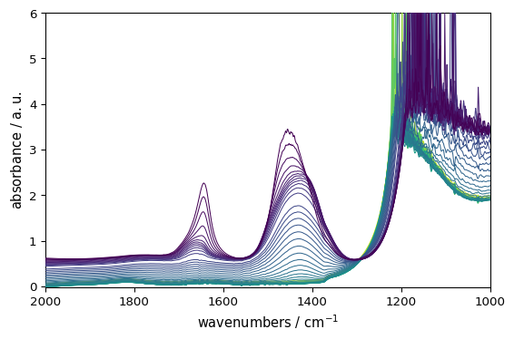
../../_images/userguide_plotting_customization_10_0.png

Axis Limits

Restrict the displayed range:

[6]:

_ = ds.plot(
    xlim=(2000, 1000)
)  # NB: slicing is also possible here, ds[:,2000.:1000.].plot() would give the same result

../../_images/userguide_plotting_customization_12_0.png

[7]:

_ = ds.plot(ylim=(0, 0.5))

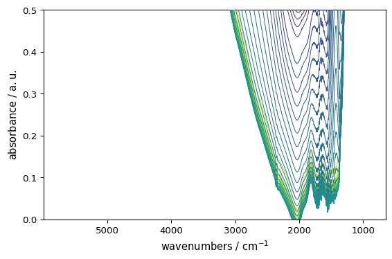
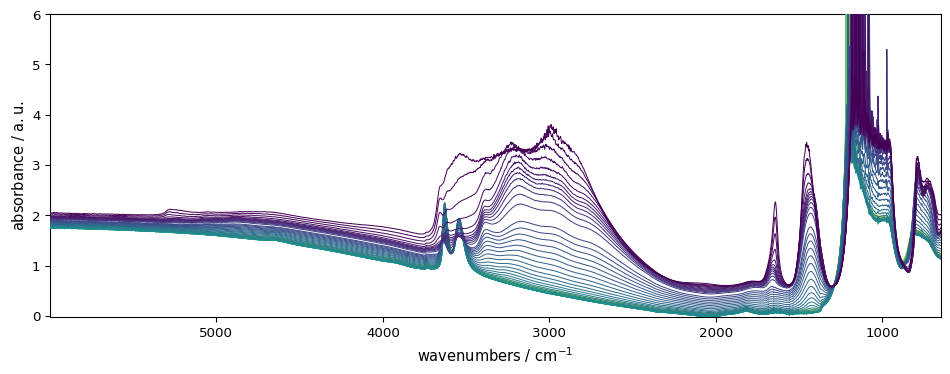
../../_images/userguide_plotting_customization_13_0.png

Figure Size

Control the figure dimensions (width, height in inches):

[8]:

_ = ds.plot(figsize=(10, 4))

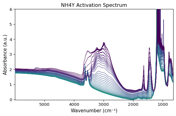
../../_images/userguide_plotting_customization_15_0.png

Titles and Labels

ds.plot() returns a Matplotlib Axes object. Use it to set titles and labels:

[9]:

ax = ds.plot()
ax.set_title("NH4Y Activation Spectrum")
ax.set_xlabel("Wavenumber (cm⁻¹)")
ax.set_ylabel("Absorbance (a.u.)")

[9]:

Text(0, 0.5, 'Absorbance (a.u.)')

../../_images/userguide_plotting_customization_17_1.png

Grid

Add a grid for easier reading:

[10]:

_ = ds.plot(grid=True)

../../_images/userguide_plotting_customization_19_0.png

Colormap

As shown in the overview, change colors using the cmap argument:

[11]:

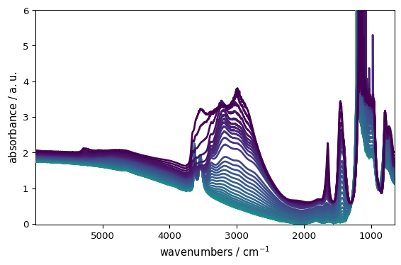
_ = ds.plot(cmap="viridis")

../../_images/userguide_plotting_customization_21_0.png

Categorical Colors (cmap=None)

For line plots, passing cmap=None uses categorical colors instead of a continuous colormap:

[12]:

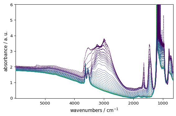
_ = ds.plot_lines(cmap=None)

../../_images/userguide_plotting_customization_23_0.png

Colormap Normalization

You can customize how colors map to values using Matplotlib’s normalization classes:

[13]:

import matplotlib as mpl

# Centered norm - useful for data with a natural center (e.g., deviations from mean)
norm = mpl.colors.CenteredNorm()
_ = ds.plot_image(cmap="RdBu_r", norm=norm)

../../_images/userguide_plotting_customization_25_0.png

Log norm - useful for data spanning several orders of magnitude norm = mpl.colors.LogNorm(vmin=0.01, vmax=1.0) _ = ds.plot_image(cmap=”viridis”, norm=norm)

Combining Customizations

Most arguments can be combined for a tailored plot:

[14]:

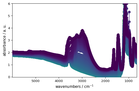
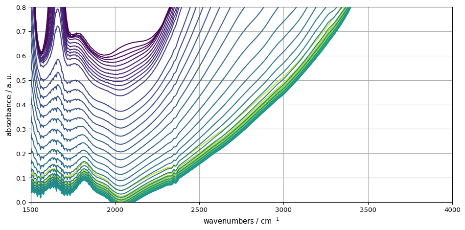
_ = ds.plot(
    xlim=(1500, 4000),
    ylim=(0, 0.8),
    linewidth=1.5,
    linestyle="-",
    grid=True,
    figsize=(10, 5),
)

../../_images/userguide_plotting_customization_28_0.png

The Mental Model

To summarize:

ds.plot() gives you a clean default.
Keyword arguments customize a single plot.
The returned Axes object provides full Matplotlib control.
Persistent changes across sessions are handled via scp.preferences (covered elsewhere).

These tools cover most day-to-day plotting needs.