Plotting Overview
SpectroChemPy plotting is designed to be:
Automatic – sensible defaults are chosen for you.
Consistent – similar data produces similar visuals.
Customizable – override anything locally or globally.
Style-driven – visual appearance can be changed without rewriting code.
In most cases, plotting your data requires only one line.
Your First Plot
Once a dataset is loaded, simply call the plot() method:
[1]:
import spectrochempy as scp
ds = scp.read("irdata/nh4y-activation.spg")
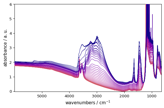
_ = ds.plot()
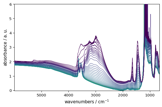
That’s it.
Here SpectroChemPy automatically:
Detects the dataset is 2D and chooses an appropriate plot type (stacked lines in this case).
Selects a suitable colormap (sequential because the y-dimension is a time axis)
Adds axis labels from dataset metadata.
Adjusts layout and scaling.
In most situations, no additional configuration is needed.
Automatic Plot Type Selection
The plot() method adapts to the dimensionality of your dataset:
Dataset type |
Default plot |
|---|---|
1D / 2D |
Line(s) plot |
2D field |
Image / contour (depending on method) |
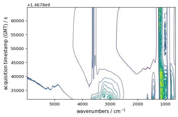
But you can also explicitly choose another plotting method:
[2]:
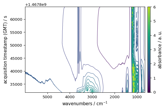
_ = ds.plot_contour()
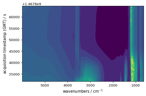
[3]:
_ = ds.plot_image()
Automatic Color Selection
SpectroChemPy chooses colors intelligently:
for lines:
Sequential data → sequential palette lines (default viridis, defined by
prefs.colormap_sequential)Categorical stacks → distinct categorical colors (default tab10 or tab20 depending on number of lines)
for contours and images:
Data with both positive and negative values → diverging colormap (default RdBu_r, defined by
prefs.colormap_diverging)Data with only positive or only negative values → sequential colormap (default viridis, defined by
prefs.colormap_sequential)
This behavior works automatically — no configuration required.
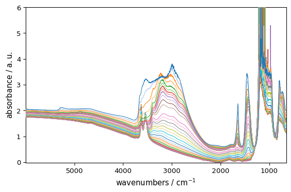
For line plots, however, you can disable continuous colormaps and force use categorical colors:
[4]:
_ = ds.plot_lines(palette="categorical")
For images and contours, you can also override the default sequential/diverging colormap behavior. Lets first have a a dataset with both positive and negative values: ds_neg = ds - ds.mean() ds_neg.plot_image(colorbar=True)
As expected,the default diverging colormap has been chosen . But this can be overriden using:
ds_neg.plot_image(cmap_mode=’sequential’) # forces sequential colormap even for data with negative values
The switch between sequential and diverging colormaps is based on the actual data values, with a diverging_margin which fixes the minimum ratio threshold for diverging auto-detection. If the data contains negative values, but they are small compared to the overall data range (i.e. they are less than diverging_margin of the data range), then a sequential colormap will be used instead of a diverging one. This prevents the use of diverging colormaps when the negative (resp. positive) values
are negligible compared to the positive (resp. negative) values, which would not provide meaningful color differentiation. The default value for diverging_margin is 0.05, meaning that if the negative values are less than 5% of the data range, a sequential colormap will be used even if there are negative values present. You can adjust this threshold as needed. For example, in the above example, setting diverging_margin=0.5 will allows for a much larger proportion of negative values (up to
50% of the data range) before switching to a diverging colormap, which is why the sequential colormap is used in this case: ds_neg.plot_image(diverging_margin=0.5)
Colorbars
By default SpectroChemPy never print a colorbar. But using the option colorbar=auto will make it print whenever a sequential or diverging colormap is used/
[5]:
_ = ds.plot_contour(colorbar="auto") # shows colorbar whenever applicable
Changing the Colormap
You can change colors per plot:
[6]:
_ = ds.plot(cmap="plasma") # note that palette="plasma" would also work for line plots
Colormap Precedence
When choosing a colormap, SpectroChemPy follows this priority order:
Explicit ``cmap`` kwarg (i.e.
cmap=XXXpassed in plot() — highest priorityPreferences colormap — if set and not “auto” (see preferences documentation)
Matplotlib style — if the style sets
image.cmapand prefs.colormap is “auto” (see styles documentation)Default preferences —
prefs.colormap_sequentialorprefs.colormap_diverging(see preferences documentation)
This means:
ds.plot(cmap="inferno")always uses infernoprefs.colormap = "cividis"uses cividis (unless overridden by explicit cmap)ds.plot(style="grayscale")withprefs.colormap="auto"uses grayscaleDefault behavior uses preferences-defined sequential/diverging colormaps
Changing the Overall Style
You can change the visual appearance using styles:
[7]:
_ = ds.plot(style="grayscale")
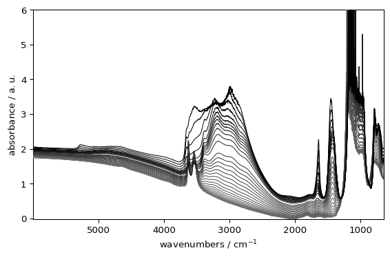
Styles can affect fonts, grid appearance, backgrounds, and (in auto mode) colormap defaults. When passes in a plot() function the change is on a ped-plot basis. You can also set a style globally and persistently using scp.preferences.style, which will affect all subsequent plots.
The Mental Model
In practice:
ds.plot()just works.cmap=(orpalette=for lines) changes colors.colorbar=controls the colorbar.style=changes the overall appearance.scp.preferenceschanges defaults persistently.
Everything else is optional.
In the following sections, we will explore how to customize plots in more detail.