× ⚠️ You are reading the development version documentation.
Read here the documentation of the last stable release.

Integrate a baseline-corrected IR band

This example shows how to baseline-correct a spectral region and compare trapezoidal and Simpson integration on a sequence of IR spectra.

import spectrochempy as scp

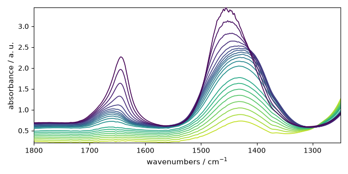
Load a stacked IR dataset and restrict the analysis to the band of interest.

dataset = scp.read_omnic("irdata/nh4y-activation.spg")
band = dataset[:20, 1250.0:1800.0]
band.y -= band.y[0]
band.y.ito("min")
band.y.title = "acquisition time"

prefs = scp.preferences
prefs.figure.figsize = (7, 3.5)
prefs.colormap = "Dark2"
prefs.colorbar = True
_ = band.plot()

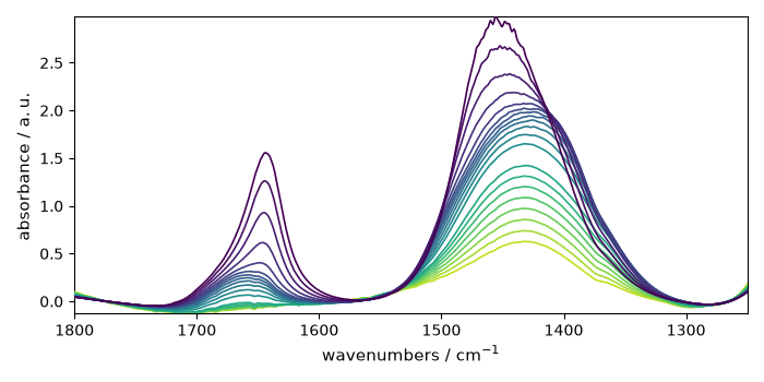
Fit a polynomial baseline on three reference regions.

blc = scp.Baseline(model="polynomial", order=3)
blc.ranges = (
    [1740.0, 1800.0],
    [1550.0, 1570.0],
    [1250.0, 1300.0],
)
blc.fit(band)

corrected = blc.corrected
_ = corrected.plot()

Integrate each spectrum over the full selected region.

trapz_area = corrected.trapezoid(dim="x")
simpson_area = corrected.simpson(dim="x")

scp.plot_multiple(
    method="scatter",
    ms=5,
    datasets=[trapz_area, simpson_area],
    labels=["trapezoidal rule", "Simpson's rule"],
    legend="best",
)

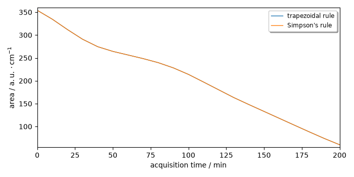
<Axes: xlabel='acquisition time $\\mathrm{/\\ \\mathrm{min}}$', ylabel='area $\\mathrm{/\\ \\mathrm{a.u.} \\cdot \\mathrm{cm}^{-1}}$'>

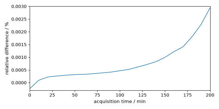
For this dataset both numerical methods are very close.

relative_difference = (trapz_area - simpson_area) * 100.0 / simpson_area
relative_difference.title = "relative difference"
relative_difference.units = "percent"
_ = relative_difference.plot(scatter=True, ms=5)

This ends the example. Uncomment the next line to display the figures when running the script directly with Python.

# scp.show()