Slice an NDDataset with indices and coordinates

This example shows how to combine standard Python slicing with coordinate-aware slicing on an infrared time series.

import spectrochempy as scp

Load and inspect the dataset

dataset = scp.read_omnic(
    "irdata/CO@Mo_Al2O3.SPG",
    description="CO adsorption, difference spectra",
)
dataset.y = (dataset.y - dataset[0].y).to("minute")
dataset
NDDataset [CO@Mo_Al2O3] — float64, shape: (y:19, x:3112), a.u.
name
:
CO@Mo_Al2O3
author
:
runner@runnervmzvulz
created
:
2026-08-18 21:26:04+00:00
description
:
CO adsorption, difference spectra
history
:
2026-08-18 21:26:04+00:00> Imported from spg file /home/runner/.spectrochempy/testdata/irdata/CO@Mo_Al2O3.SPG.
2026-08-18 21:26:04+00:00> Sorted by date
Data
title
:
absorbance
values
:
[[0.0008032 3.788e-05 ... 0.0003027 0.0003745]
[-3.608e-05 -0.0001981 ... 0.0003089 0.00117]
...
[0.0008357 -0.0001387 ... -0.0005221 -0.001121]
[0.0005655 -0.000116 ... -0.00057 -0.0006307]] a.u.
shape
:
(y:19, x:3112)
Dimension `x`
size
:
3112
title
:
wavenumbers
coordinates
:
[ 4000 3999 ... 1001 999.9] cm⁻¹
Dimension `y`
size
:
19
title
:
acquisition timestamp (GMT)
coordinates
:
[ 0 4.517 ... 132 137] min
labels
:
[[ 2016-10-18 13:49:35+00:00 2016-10-18 13:54:06+00:00 ... 2016-10-18 16:01:33+00:00 2016-10-18 16:06:37+00:00]
[ *Résultat de Soustraction:04_Mo_Al2O3_calc_0.003torr_LT_after sulf_Oct 18 15:46:42 2016 (GMT+02:00)
*Résultat de Soustraction:04_Mo_Al2O3_calc_0.004torr_LT_after sulf_Oct 18 15:51:12 2016 (GMT+02:00) ...
*Résultat de Soustraction:04_Mo_Al2O3_calc_0.905torr_LT_after sulf_Oct 18 17:58:42 2016 (GMT+02:00)
*Résultat de Soustraction:04_Mo_Al2O3_calc_1.004torr_LT_after sulf_Oct 18 18:03:41 2016 (GMT+02:00)]]


prefs = scp.preferences
prefs.figure.figsize = (7, 4)
_ = dataset.plot()
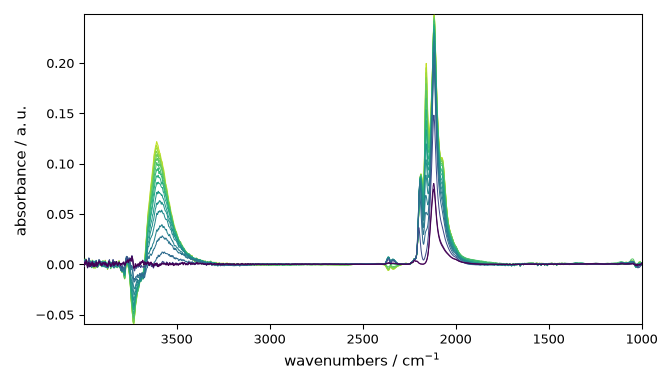
plot d slicing

Integer-based slicing

Standard integer slices work as expected on both dimensions:

(4, 3112)
(19, 1556)

Coordinate-aware slicing

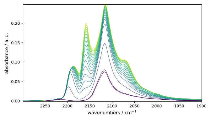
Using floats slices directly on axis coordinates instead of integer indices:

plot d slicing

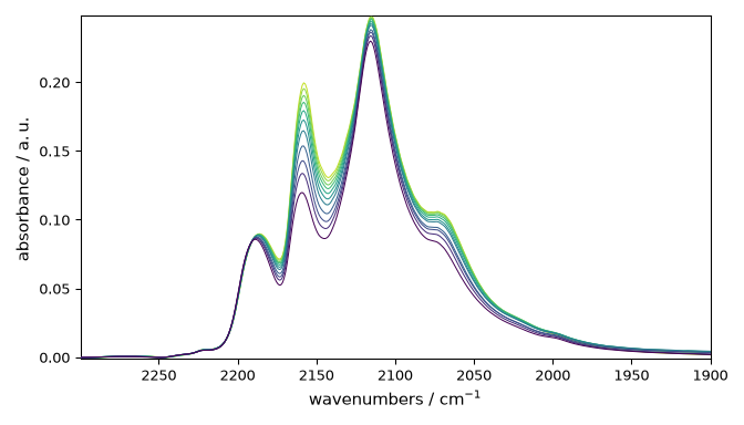
The same applies to the time axis:

window = dataset[80.0:137.0, 2300.0:1900.0]
_ = window.plot()
plot d slicing

Selecting the closest spectrum

A single float selects the nearest spectrum on that axis:

Coord [y:acquisition timestamp (GMT)] — float64, size: 1, min
size
:
1
title
:
acquisition timestamp (GMT)
coordinates
:
[ 58.32] min
labels
:
[[ 2016-10-18 14:47:54+00:00]
[ *Résultat de Soustraction:04_Mo_Al2O3_calc_0.021torr_LT_after sulf_Oct 18 16:45:00 2016 (GMT+02:00)]]


This ends the example. Uncomment the next line to display the figures when running the script directly with Python.

# scp.show()

Total running time of the script: (0 minutes 0.524 seconds)