Note
Go to the end to download the full example code.
Two-dimensional NMR processing
Temporarily excluded from the public gallery.
This source is preserved for the future 2D characterization campaign, but the
current public NMR workflow intentionally supports only validated 1D
processing. On the merged public branch, scp.nmr.Experiment.process()
raises NotImplementedError for multi-dimensional datasets, so this example is
not published while 2D support remains under separate scientific review.
This example complements sphx_glr_plugins_spectrochempy-nmr_examples_processing_nmr_plot_processing_nmr.py:
plot_processing_nmr.pystarts from a TopSpin2rrdataset that is already processed.This example starts from the raw TopSpin
serfile and performs the main processing steps inside SpectroChemPy.
The pipeline is intentionally split in two stages:
F2 (direct dimension): apodization -> FFT -> auto-phase
F1 (indirect dimension): zero-filling -> apodization -> FFT
It illustrates:
reading raw 2D SER data;
automatic handling of Bruker encodings such as
STATES-TPPI;quaternion-aware 2D FFT processing;
how to obtain a spectrum comparable to the processed
2rrreference.
Requires the official spectrochempy-nmr plugin.
Install with: pip install spectrochempy[nmr].
Import API
import spectrochempy as scp
Read raw 2D SER data
The raw SER file contains time-domain data together with the acquisition metadata needed to decode the hypercomplex encoding in F1.
nmrdir = scp.preferences.datadir / "nmrdata" / "bruker" / "tests" / "nmr"
ser = scp.nmr.read(nmrdir / "topspin_2d", expno=1, remove_digital_filter=True)
/home/runner/work/spectrochempy/spectrochempy/plugins/spectrochempy-nmr/src/spectrochempy_nmr/extern/nmrglue/_bruker.py:441: UserWarning: (196608,)cannot be shaped into(147, 1024)
  _, data = read_binary(f, shape=shape, cplex=cplex, big=big, isfloat=isfloat)
Print dataset summary — both dimensions are in time domain
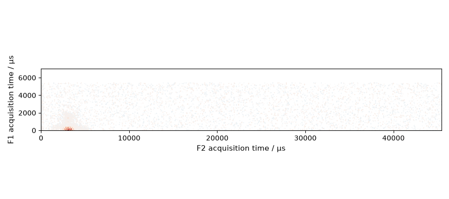
Plot the raw time-domain data (quaternion representation)
For comparison, load the TopSpin-processed reference spectrum.
This is similar to the dataset used in plot_processing_nmr.py.
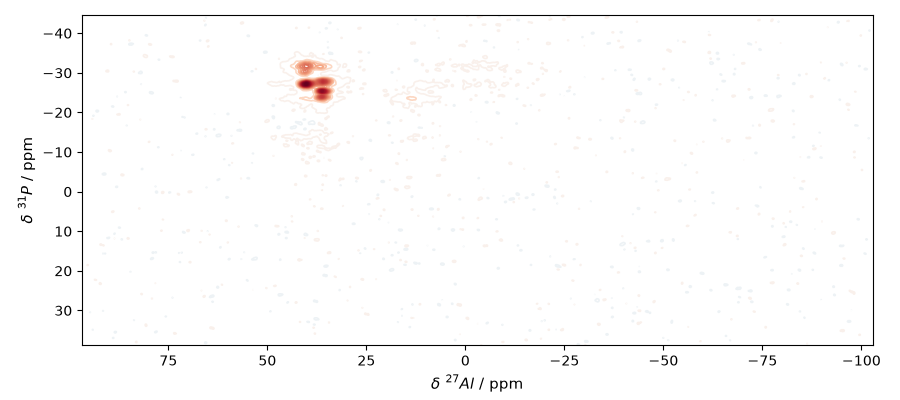
reference = scp.nmr.read(nmrdir / "topspin_2d" / "1" / "pdata" / "1" / "2rr")
Plot the processed TopSpin reference
Stage 1: process F2 (direct dimension)
Experiment.process() applies the usual direct-dimension workflow:
exponential multiplication, FFT, then automatic phasing along F2.
Here we also set the F2 zero-filled size to match the processed TopSpin spectrum more closely.
from spectrochempy_nmr import Experiment

exp = Experiment(ser)
f2_processed = exp.process(apodization="em", lb=2.0, size=2048)

# After F2 processing: F2 is in frequency domain, F1 is still time domain
f2_processed
Traceback (most recent call last):
  File "/home/runner/work/spectrochempy/spectrochempy/build/~gallery_examples/processing/nmr/plot_processing_nmr_2d.py", line 86, in <module>
    f2_processed = exp.process(apodization="em", lb=2.0, size=2048)
  File "/home/runner/work/spectrochempy/spectrochempy/plugins/spectrochempy-nmr/src/spectrochempy_nmr/experiment.py", line 545, in process
    raise NotImplementedError(msg)
NotImplementedError: Public NMR processing currently supports only validated 1D experiments. Multi-dimensional NMR processing remains out of public scope pending further scientific characterization.
Plot after F2 processing — only the horizontal axis is transformed
_ = f2_processed.plot_map()
Stage 2: process F1 (indirect dimension)
F1 still needs the usual indirect-dimension steps. We keep them explicit here because they are often tuned case by case in practice.
The values below are chosen so that the resulting spectrum is close to the
processed TopSpin 2rr reference shipped with the test data.
f1 = f2_processed.zf_size(size=1024, dim="y")
f1 = f1.em(lb=5.0, dim="y")
f1 = f1.fft(dim="y")

f1
Plot the fully processed 2D spectrum
_ = f1.plot_map()
Extract and inspect a 1D slice
Once the 2D spectrum is processed we can reuse the same style of operations
shown in plot_processing_nmr.py.
slice_f2 = f1[-27.6, :]
_ = slice_f2.plot()
Compare the same slice against the TopSpin 2rr reference.
We normalize both traces before overlaying them because the absolute
intensity depends on the exact processing chain (window functions,
phasing, scaling conventions, etc.).
Total running time of the script: (0 minutes 3.228 seconds)